
Analysis plays a role at every point in the process of designing and implementing algorithms. At first, as we saw, we can save factors of thousands or millions in the running time with appropriate algorithm design choices. As we consider more efficient algorithms, we find it more of a challenge to choose among them, so we need to study their properties in more detail. In pursuit of the best ( in some precise technical sense ) algorithm, we find both algorithms that are useful in practice and theoretical questions that are challenging to resolve.
It is worthwhile for us to consider the basics of methods for the analysis of algorithms here, so that we can
- Illustrate the process.
- Describe in one place the mathematical conventions that we use.
- Provide a basis for discussion of higher-level issues.
- Develop an appreciation for scientific underpinnings of the conclusions that we draw when comparing algorithms.
Most important, algorithms and their analysis are often intertwined.
1、Implementation and Empirical Analysis
if an algorithm is to be implemented as part of a large system, we use abstract data types or a similar mechanism to make it possible to change algorithms or implementations after we determine what part of the system deserves the most attention. From the start, however, we need to have an understanding of each algorithm’s performance characteristics, because design requirements of the system may have a major influence on algorithm performance. Such initial design decisions must be made with care, because it often does turn out, in the end, that the performance of the whole system depends on the performance of some basic algorithm.
One of the first steps that we take to understand the performance of algorithms is to do empirical analysis. Given two algorithms to solve the same problem, there is no mystery in the method: We run them both to see which one takes longer!
When empirical studies start to consume a significant amount of time, mathematical analysis is called for.
The first challenge that we face in empirical analysis is to develop a correct and complete implementation.
The second challenge that we face in empirical analysis is to determine the nature of the input data and other factors that have direct influence on the experiments to be performed. Typically, we have three basic choices: use actual data, random data, or perverse data. Actual data enable us truly to measure the cost of the program in use; random data assure us that our experiments test the algorithm, no the data; and perverse data assure us that our programs can handle any input presented them.
Perhaps the most common mistake made in selecting an algorithm is to ignore performance characteristics. Faster algorithms are often more complicated than brute-force solutions, and performers are often willing to accept a slower algorithm to avoid having to deal with added complexity.
Perhaps the second most common mistake made in selecting an algorithm is to pay too much attention to performance characteristics.
2、Analysis of Algorithms
The following are among the reasons that we perform mathematical analysis of algorithms:
- To compare different algorithms for the same task
- To predict performance in a new environment
- To set values of algorithm parameters
Several important factors in a precise analysis are usually outside a given programmer’s domain of influence.
First, C programs are translated into machine code for a given computer, and it can be a challenging task to figure out exactly how long even one C statement might take to execute ( especially in an environment where resources are being shared, so even the same program can have varying performance characteristics at two different times ).
Second, many programs are extremely sensitive to their input data, and performance might fluctuate wildly depending on the input.
Third, many programs of interest are not well understood, and specific mathematical results may not be available.
Finally, two programs might not be comparable at all: one may run much more efficiently on one particular kind of input, the other runs efficiently under other circumstances.
All these factors notwithstanding, it is often possible to predict precisely how long a particular program will take, or to know that one program will do better than another in particular situations. Moreover, we can often acquire such knowledge by using one of a relatively small set of mathematical tools.
The first step in the analysis of an algorithm is to identify the abstract operations on which the algorithm is based, to separate the analysis from the implementation.
We also have to study the data, and to model the input that might be presented to the algorithm. Most often, we consider one of two approaches to the analysis: we either assume that the input is random, and study the average-case performance of the program, or we look for perverse input, and study the worst-case performance of the program.
3、Growth of Functions
Most algorithms have a primary parameter N that affects the running time most significantly. The parameter N might be the degree of a polynomial, the size of a file to be sorted or searched, the number of characters in a text string, or some other abstract measure of the size of the problem being considered: it is most often directly proportional to the size of the data set being processed.
Our goal is to express the resource requirements of our programs (most often running time ) in terms of N, using mathematical formulas that are as simple as possible and that are accurate for large values of the parameters.
The algorithms typically have running times proportional to one of the following functions:
1 Most instructions of most programs are executed once or at most only a few times. If all the instructions of a program have this property, we say that the program’s running time is constant.
log N When the running time of a program is logarithmic, the program gets slightly slower as N grows. This running time commonly occurs in programs that solve a big problem by transformation into a series of smaller problems, cutting the problem size by some constant fraction at each step. For our range of interest, we can consider the running time to be less than a large constant.
N When the running time of a program is linear, it is generally the case that a small amount of processing is done on each input element.
N log N The N log N running time arises when algorithms solve a problem by breaking it up into smaller sub-problems, solving them independently, and then combining the solutions. For lack of a better adjective, we simply say that the running time of such an algorithm is N log N.
N2 When the running time of an algorithm is quadratic, that algorithm is practical for use on only relatively small problems. Quadratic running times typically arise in algorithms that process all pairs of data items ( perhaps in a double nested loop ).
N3 Similarly, an algorithm that processes triples of data items ( perhaps in a triple-nested loop ) has a cubic running time and is practical for use on only small problems.
2N Few algorithms with exponential running time are likely to be appropriate for practical use, even though such algorithms arise naturally as brute-force solutions to problems.
The running time of a particular program is likely to be some constant multiplied by one of these terms ( the leading term ) plus some smaller terms. The value of the constant coefficient and the terms included depend on the results of the analysis and on implementation details. Roughly, the coefficient of the leading term has to do with the number of instructions in the inner loop: At any level of algorithm design, it is prudent to limit the number of such instructions. For large N, the effect of the leading term dominates; for small N or for carefully engineered algorithms, more terms may contribute and comparisons of algorithms are more difficult.
In most cases, we will refer to the running time of programs simply as “linear”, “N log N”, “cubic”, and so forth.
Time to solve huge problems: A fast algorithm enables us to solve a problem on a slow machine, but a fast machine is no help when we are using a slow algorithm.
Eventually, to reduce the total running time of a program, we focus on minimizing the number of instructions in the inner loop. Each instruction comes under scrutiny: Is it really necessary? Is there a more efficient way to accomplish the same task?
The logarithm function plays a special role in the design and analysis of algorithms, so it is worthwhile for us to consider it in detail. Because we often deal with analytic results only to within a constant factor, we use the notation “log N” without specifying the base. Changing the base from one constant to another changes the value of the logarithm by only a constant factor, but specific bases normally suggest themselves in particular contexts.
In mathematics, the natural logarithm ( base e = 2.71828… ) is so important that a special abbreviation is commonly used: loge N ≡ ln N. In computer science, the binary logarithm ( base 2 ) is so important that the abbreviation log2 N ≡ lg N is commonly used.
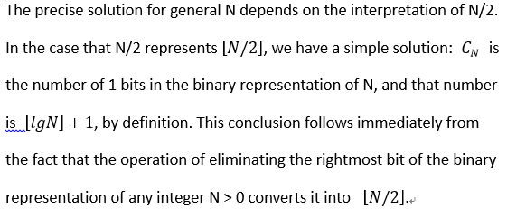
Rounded up to the nearest integer, lg N is the number of bits required to represent N in binary, in the same way that log10 N rounded up to the nearest integer is the number of digits required to represent N in decimal.
The C statement
for (lg N = 0; N > 0; lg N ++; N /= 2) ;
is a simple way to compute the smallest integer larger than lg N.
A similar method for computing this function is
for (lg N = 0, t = 1; t < N; lg N++, t += t);
This version emphasizes that 2n ≤ N < 2n+1 when n is the smallest integer larger than lg N. We also frequently encounter a number of special functions and mathematical notations from classical analysis that are useful in providing concise descriptions of properties of programs. Table 1 summarizes the most familiar for these functions; we briefly discuss them and some of their most important properties in the following paragraphs.
Table 1 Special functions and constants
This table summarizes the mathematical notation that we use for functions and constants that arise in formulas describing the performance of algorithms. The formulas for the approximate values extend to provide much more accuracy, if desired.
Our algorithms and analyses most often deal with discrete units, so we often have need for the following special functions to convert real numbers to integers:
![]()
![]() 4、Big-Oh Notation
4、Big-Oh Notation
The mathematical artifact that allows us to suppress detail when we are analyzing algorithms is called the O-notation, or “big-Oh notation”, which is defined as follows.
Definition 1 A function g(N) is said to be O(f(N)) if there exist constants c0 and N0 such that g(N) is less than c0f(N) for all N > N0.
We use the O-notation for three distinct purpose:
- To bound the error that we make when we ignore small terms in mathematical formulas
- To bound the error that we make when we ignore parts of a program that contribute a small amount to the total being analyzed
- To allow us to classify algorithms according to upper bounds on their total running times
Often, the results of a mathematical analysis are not exact, but rather are approximate in a precise technical sense: The result might be an expression consisting of a sequence of decreasing terms. Just as we are most concerned with the inner loop of a program, we are most concerned with the leading terms (the largest terms) of a mathematical expression.
The O-notation allows us to keep track of the leading terms while ignoring smaller terms when manipulating approximate mathematical expressions, and ultimately allows us to make concise statements that give accurate approximations to the quantities that we analyze.
Essentially, we can expand algebraic expressions using the O-notation as though the O were not there, then can drop all but the largest term. For example, if we expand the expression
(N + O(1))(N + O(log N) + O(1)),
we get six terms
N2 + O(N) + O(N log N) + O(log N) + O(N) + O(1),
but can drop all but the largest O-term, leaving the approximation
N2 + O(N log N).
That is, N2 is a good approximation to this expression when N is large. These manipulations are intuitive, but the O-notation allows us to express them mathematically with rigor and precision. We refer to a formula with one O-term as an asymptotic expression.
We use O-notation primarily to learn the fundamental asymptotic behavior of an algorithm; is proportional to when we want to predict performance by extrapolation from empirical studies; and about when we want to compare performance or to make absolute performance predictions.
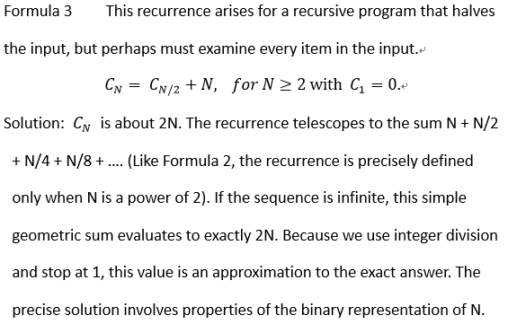
5、Basic Recurrences
A great many algorithms are based on the principle of recursively decomposing a large problem into one or more smaller ones, using solutions to the sub-problems to solve the original problem.
Understanding the mathematical properties of the formulas in this section will give us insight into the performance properties of algorithms.
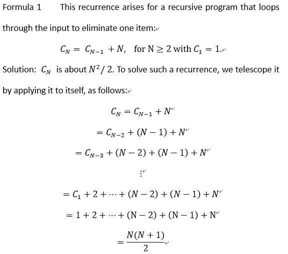
Evaluating the sum 1 + 2 + … + (N -2) + (N-1) + N is elementary: The given result follows when we add the sum to itself, but in reverse order, term by term. This result—twice the value sought—consists of N terms, each of which sums to N + 1.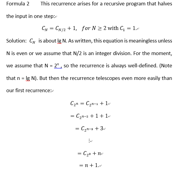
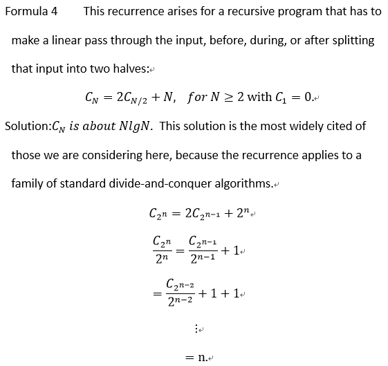 We develop the solution very much as we did in Formula 2, but with the additional trick of dividing both sides of the recurrence by 2n at the second step to make the recurrence telescope.
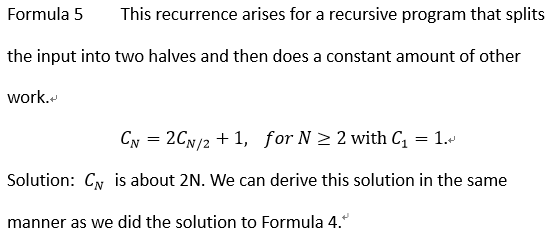
We can solve minor variants of these formulas, involving different initial conditions of slight differences in the additive term, using the same solution techniques, although we need to be aware that some recurrences that seem similar to these may actually be rather difficult to solve. There is a variety of advanced general techniques for dealing with such equations with mathematical rigor. We will encounter a few more complicated recurrences in the future, but we defer discussion of their solution until they arise.