
In this series, we continue our study of SQL. We consider more complex forms of SQL queries, view definition, transactions, integrity constrains, more details regarding SQL data definition, and authorization.1、Join Expressions
In Relational Databases ~ Introduction to SQL II, we introduced the natural join operation. SQL provides other forms of the join operation, including the ability to specify an explicit join predicate, and the ability to include in the result tuples that are excluded by natural join. We shall discuss these forms of join in this section.
The examples in this section involve the two relations student and takes, shown in Figure 1 and 2, respectively. Observe that the attribute grade has a value null for the student with ID 98988, for the course BIO-301, section 1, taken in Summer 2010. The null value indicates that the grade has not been awarded yet.
 Figure 1 The student relationFigure 2 The takes relation
1.1 Join Conditions
In Relational Databases ~ Introduction to SQL II, we saw how to express natural joins, and we saw the join … using clause, which is a form of natural join that only requires values to match on specified attributes. SQL supports another form of join, in which an arbitrary join condition can be specified.
The on condition allows a general predicate over the relations being joined. This predicate is written like a where clause predicate except for the use of the keyword on rather than where. Like the using condition, the on condition appears at the end of the join expression. Consider the following query, which has a join expression containing the on condition. The on condition above specifies that a tuple from student matches a tuples from takes if their ID values are equal. The join expression in this case is almost the same as the join expression student natural join takes, since the natural join operation also requires that for a student tuple and a takes tuple to match. The one difference is that the result has the ID attribute listed twice, in the join result, once for the student and once for takes, even though their ID values must be the same.
In fact, the above query is equivalent to the following query (in other words, they generate exactly the same results): As we have seen earlier, the relation name is used to disambiguate the attribute name ID, and thus the two occurrences can be referred to as student.ID and takes.ID respectively. A version of this query that displays the ID value only once is as follows:
 Figure 3 The result of student join takes on student.ID=takes.ID with second occurrence of ID omitted.
The on condition can express any SQL predicate, and thus a join expressions using the on condition can express a richer class of join conditions than natural join. However, as illustrated by our preceding example, a query using a join expression with an on condition can be replaced by an equivalent expression without the on condition, with the predicate in the on clause moved to the where clause. Thus, it may appear that the on condition is a redundant feature of SQL.
However, there are two good reasons for introducing the on condition. First, we shall see shortly that for a kind of join called an outer join, on conditions do behave in a manner different from where conditions. Second, an SQL query is often more readable by humans if the join condition is specified in the on clause and the rest of the conditions appear in the where clause.
1.2 Outer Joins
Suppose we wish to display a list of all students, displaying their ID, and name, dept_name, and tot_cred, along with the courses that they have taken. The following SQL query may appear to retrieve the required information: Unfortunately, the above query does not work quite as intended. Suppose that there is some student who takes no courses. Then the tuple in the student relation for that particular student would not satisfy the condition of a natural join with any tuple in the take relation, and that student’s data would not appear in the result. We would thus not see any information about students who have not taken any course. For example, in the student and takes relations of Figure 1 and 2, note that student Snow, with ID 70557, has not taken any courses. Snow appears in student, but Snow’s ID number does not appear in the ID column of takes. Thus, Snow does not appear in the result of the natural join.
More generally, some tuples in either or both of the relations being joined may be “lost” in this way. The outer join operation works in a manner similar to the join operations we have already studied, but preserve those tuples that would be lost in a join, by creating tuples in the result containing null values.
For example, to ensure that the student named Snow from our earlier example appears in the result, a tuple could be added to the join result with all attributes from the student relation set to the corresponding values for the student Snow, and all the remaining attributes which come from the takes relation, namely course_id, sec_id, semester, and year, set to null. Thus the tuple for the student Snow is preserved in the result of the outer join. There are in fact three forms of outer join:
- The left outer join preserves tuples only in the relation named before (to the left of) the left outer join operation.
- The right outer join preserves tuples only in the relation named after (to the right of) the right outer join operation.
- The full outer join preserves tuples in both relations.
In contrast, the join operations we studied earlier that do not preserve nonmatched tuples are called inner join operations, to distinguish them from the outer-join operations. We now explain exactly how each form of outer join operates. We can compute the left outer-join operation as follows. First, compute the result of the inner join as before. Then, for every tuple t in the left-hand-side relation that does not match any tuple in the right-hand-side relation in the inner join, add a tuple r to the result of the join constructed as follows:
- The attributes of tuple r that are derived from the left-hand-side relation are filled in with the values from tuple t.
- The remaining attributes of r are filled with null values.
 Figure 4 Result of student natural left outer join takes.
The result includes student Snow (ID 70557), unlike the result of an inner join, but the tuple for Snow includes nulls for the attributes that appear only in the schema of the takes relation. As another example of the use of the outer-join operation, we can write the query “Find all students who have not taken a course” as: The right outer join is symmetric to the left outer join. Tuples from the right-hand-side relation that do not match any tuple in the left-hand-side relation are padded with nulls and are added to the result of the right outer join. Thus, if we rewrite our above query using a right outer join and swapping the order in which we list the relations as follows:
 Figure 5 The result of takes natural right outer join student.
The full outer join is a combination of the left and right outer-join types. After the operation computes the result of the inner join, it extends with nulls those tuples from the left-hand-side relation that did not match with any from the right-hand side relation, and adds them to the result. Similarly, it extends with nulls those tuples from the right-hand-side relation that did not match with any tuples from the left-hand-side relation and adds them to the result.
The on clause can be used with outer joins. The following query is identical to the first query we saw using “student natural left outer join takes,” except that the attribute ID appears twice in the result. As we noted earlier, on and where behave differently for outer join. The reason for this is that outer join adds null-padded tuples only for those tuples that do not contribute to the result of the corresponding inner join. The on condition is part of the outer join specification, but a where clause is not. In our example, the case of the student tuple for student “Snow” with ID 70557, illustrates this distinction. Suppose we modify the preceding query by moving the on clause predicate to the where clause, and instead using an on condition of true.
 The earlier query, using the left outer join with the on condition, includes a tuple(70557,Snow,Physics,0,null,null,null,null,null,null), because there is no tuple in takes with ID = 70557. In the later query, however, every tuple satisfies the join condition true, so no null-padded tuples are generated by the outer join. The outer join actually generates the Cartesian product of the two relations. Since there is no tuple in takes with ID=70557, every time a tuple appears in the outer join with name = “Snow”, the values for student.ID and takes.ID must be different, and such tuples would be eliminated by the where clause predicate. Thus student Snow never appears in the result of the latter query.
1.3 Join Types and Conditions
To distinguish normal joins from outer joins, normal joins are called inner joins in SQL. A join clause can thus specify inner join instead of outer join to specify that a normal join is to be used. The keyword inner is, however, optional. The default join type, when the join clause is used without the outer prefix is the inner join. Thus, is equivalent to:
 Similarly, natural join is equivalent to natural inner join.
 Figure 4.6 Join types and join conditions.
Figure 4.6 shows a full list of the various types of join that we have discussed. As can be seen from the figure, any form of join (inner, left outer, right outer, or full outer) can be combined with any join condition (natural, using, or on).
2、Views
In our examples up to this point, we have operated at the logical-model level. That is, we have assumed that the relations in the collection we are given are the actual relations stored in the database. It is not desirable for all users to see the entire logical model. Security considerations may require that certain data be hidden from users. Consider a clerk who needs to know an instructor’s ID, name and department name, but does not have authorization to see the instructor’s salary amount. This person should see a relation described in SQL, by: Aside from security concerns, we may wish to create a personalized collection of relations that is better matched to a certain user’s intuition than is the logical model. We may want to have a list of all course sections offered by the Physics department in the Fall 2009 semester, with the building and room number of each section. The relation that we would create for obtaining such a list is:
It is possible to complete and store the results of the above queries and then make the stored relations available to users. However, if we did so, and the underlying data in the relations instructor, course, or section changes, the stored query results would then no longer match the result of reexecuting the query on the relations. In general, it is a bad idea to compute and store query results such as those in the above examples.
Instead, SQL allows a “virtual relation” to be defined by a query, and the relation conceptually contains the result of the query. The virtual relation is not precomputed and stored, but instead is computed by executing the query whenever the virtual relation is used. Any such relation that is not part of the logical model, but is made visible to a user as a virtual relation, is called a view. It is possible to support a large number of views on top of any given set of actual relations.
2.1 View Definition
We define a view in SQL by using the create view command. To define a view, we must give the view a name and must state the query that computes the view. The form of the create view command is: create view υ as <query expression>; where <query expression> is any legal query expression. The view name is represented by υ.
Consider again the clerk who needs to access all data in the instructor relation, except salary. The clerk should not be authorized to access the instructor relation. Instead, a view relation faculty can be made available to the clerk, with the view defined as follows:![]()
 As explained earlier, the view relation conceptually contains the tuples in the query result, but is not precomputed and stored. Instead, the database system stores the query expression associated with the view relation. Whenever the view relation is accessed, its tuples are created by computing the query result. Thus, the view relation is created whenever needed, on demand.
To create a view that lists all course sections offered by the Physics department in the Fall 2009 semester with the building and room number of each section, we write:
 2.2 Using Views in SQL Queries
Once we have defined a view, we can use the view name to refer to the virtual relation that the view generates. Using the view physics_fall_2009, we can find all Physics courses offered in the Fall 2009 semester in the Watson building by writing: View names may appear in a query any place where a relation name may appear, The attribute names of a view can be specified explicitly as follows:
![]() The preceding view gives for each department the sum of the salaries of all the instructors at that department. Since the expression sum(salary) does not have a name, the attribute name is specified explicitly in the view definition.
The preceding view gives for each department the sum of the salaries of all the instructors at that department. Since the expression sum(salary) does not have a name, the attribute name is specified explicitly in the view definition.
Intuitively, at any given time, the set of tuples in the view relation is the result of evaluation of the query expression that defines the view. Thus, if a view relation is computed and stored, it may become out of date if the relations used to define it are modified. To avoid this, views are usually implemented as follows. When we define a view, the database system stores the definition of the view itself, rather than the result of evaluation of the query expression that defines the view. Wherever a view relation appears in a query, it is replaced by the stored query expression. Thus, whenever we evaluate the query, the view relation is recomputed.
One view can’t be used in the expression defining another view in MySQL. For example, we can define a view physics_fall_2009_watson that lists the course ID and room number of all Physics courses offered in the Fall 2009 semester in the Watson building as follows:![]() where physics_fall_2009_watson is itself a view relation. This is not equivalent to in MySQL:
where physics_fall_2009_watson is itself a view relation. This is not equivalent to in MySQL:
2.3 Materialized Views
Certain database systems allow view relations to be stored, but they make sure that, if the actual relations used in the view definition change, the view is kept up-to-date. Such views are called materialized views. For example, consider the view departments_total_salary. If the above view is materialized, its result would be stored in the database. However, if an instructor tuple is added to or deleted from the instructor relation, the result of the query defining the view would change, and as a result the materialized view’s contents must be updated. Similarly, if an instructor’s salary is updated, the tuple in departments_total_salary corresponding to that instructor’s department must be updated.
The process of keeping the materialized view up-to-date is called materialized view maintenance (or often, just view maintenance) and is covered later. View maintenance can be done immediately when any of the relations on which the view is defined is updated. Some database systems, however, perform view maintenance lazily, when the view is accessed. Some systems update materialized views only periodically; in this case, the contents of the materialized view may be stale, that is, not up-to-date, when it is used, and should not be used if the application needs up-to-date data. And some database systems permit the database administrator to control which of the above methods is used for each materialized view.
Applications that use a view frequently may benefit if the view is materialized. Applications that demand fast response to certain queries that compute aggregates over large relations can also benefit greatly by creating materialized views corresponding to the queries. In this case, the aggregated result is likely to be much smaller than the large relations on which the view is defined; as a result the materialized view can be used to answer the query very quickly, avoiding reading the large underlying relations. Of course, the benefits to queries from the materialization of a view must be weighed against the storage costs and the added overhead for updates.
SQL does not define a standard way of specifying that a view is materialized, but many database systems provide their own SQL extensions for this task. Some database systems always keep materialized views up-to-date when the underlying relations change, while others permit them to become out of date, and periodically recompute them.
2.4 Update of a View
Although views are a useful tool for queries, they present serious problems if we express updates, insertions, or deletions with them. The difficulty is that a modification to the database expressed in terms of a view must be translated to a modification to the actual relations in the logical model of the database.
Suppose the view faculty, which we saw earlier, is made available to a clerk. Since we allow a view name to appear wherever a relation name is allowed, the clerk can write:![]() This insertion must be represented by an insertion into the relation instructor, since instructor is the actual relation from which the database system constructs the view faculty. However, to insert a tuple into instructor, we must have some value for salary. There are two reasonable approaches to dealing with this insertion:
This insertion must be represented by an insertion into the relation instructor, since instructor is the actual relation from which the database system constructs the view faculty. However, to insert a tuple into instructor, we must have some value for salary. There are two reasonable approaches to dealing with this insertion:
- Reject the insertion, and return an error messages to the user.
- Insert a tuple (‘30765′,’Green’,’Music’,null) into the instructor relation.
Another problem with modification of the database through views occurs with a view such as: This view lists the ID, name, and building-name of each instructor in the university. Consider the following insertion through this view:
![]() Suppose there is no instructor with ID 69987, and no department in the Taylor building. Then the only possible method of inserting tuples into the instructor and department relations is to insert (‘69987′,’White’,null,null) into instructor and (‘Chemistry’,’Taylor’,null) into department. Then, we obtain the relations shown in Figure 4.7. However, this update does not have the desired effect, since the view relation instructor_info still does not include the tuple (‘69987′,’White’,’Taylor’). Thus, there is no way to update the relations instructor and department by using nulls to get the desired update on instructor_info.
Suppose there is no instructor with ID 69987, and no department in the Taylor building. Then the only possible method of inserting tuples into the instructor and department relations is to insert (‘69987′,’White’,null,null) into instructor and (‘Chemistry’,’Taylor’,null) into department. Then, we obtain the relations shown in Figure 4.7. However, this update does not have the desired effect, since the view relation instructor_info still does not include the tuple (‘69987′,’White’,’Taylor’). Thus, there is no way to update the relations instructor and department by using nulls to get the desired update on instructor_info.
 Figure 4.7 Relations instructor and department after insertion of tuples.
Because of problems such as these, modifications are generally not permitted on view relations, except in limited cases. Different database systems specify different conditions under which they permit updates on view relations; see the database system manuals for details. The general problem of database modification through views has been the subject of substantial research, and the bibliographic notes provide pointers to some of this research.
In general, an SQL view is said to be updatable (that is, inserts, updates or deletes can be applied on the view) if the following conditions are all satisfied by the query defining the view:
- The from clause has only one database relation.
- The select clause contains only attribute names of the relation, and does not have any expressions, aggregates, or distinct specification.
- Any attribute not listed in the select clause can be set to null; that is, it does not have a not null constraint and is not part of a primary key.
- The query does not have a group by or having clause.
Under these constraints, the update, insert, and delete operations would be allowed on the following view: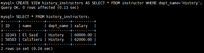 Even with the conditions on updatability, the following problem still remains. Suppose that a user tries to insert the tuple (‘25566’, ‘Brown’,’Biology’,100000) into the history_instructors view. This tuple can be inserted into the instructor relation, but it would not appear in the history_instructors view since it does not satisfy the selection imposed by the view.
By default, SQL would allow the above update to proceed. However, views can be defined with a with check option clause at the end of the view definition; then, if a tuple inserted into the view does not satisfy the view’s where clause condition, the insertion is rejected by the database system. Updates are similarly rejected if the new value does not satisfy the where clause conditions.
SQL:1999 has a more complex set of rules about when inserts, updates, and deletes can be executed on a view, that allows updates through a larger class of views; however, the rules are too complex to be discussed here.
3、Transactions
A transaction consists of a sequence of query and / or update statements. The SQL standard specifies that a transaction begins implicitly when an SQL statement is executed. One of the following SQL statements must end the transaction:
- Commit work commits the current transaction; that is, it makes the updates performed by the transaction become permanent in the database. After the transaction is committed, a new transaction is automatically started.
- Rollback work causes the current transaction to be rolled back; that is, it undoes all the updates performed by the SQL statements in the transaction. Thus, the database state is restored to what it was before the first statement of the transaction was executed.
The keyword work is optional in both the statements.
Transaction rollback is useful if some error condition is detected during execution of a transaction. Commit is similar, in a sense, to saving changes to a document that is being edited, while rollback is similar to quitting the edit session without saving changes. Once a transaction has executed commit work, its effects can no longer be undone by rollback work. The database system guarantees that in the event of some failure, such as an error in one of the SQL statements, a power outage, or a system crash, a transaction’s effects will be rolled back if it has not yet executed commit work. In the case of power outage or other system crash, the rollback occurs when the system restarts.
For instance, consider a banking application, where we need to transfer money from one bank account to another in the same bank. To do so, we need to update two account balances, subtracting the amount transferred from one, and adding it to the other. If the system crashes after subtracting the amount from the first account, but before adding it to the second account, the bank balances would be inconsistent. A similar problem would occur, if the second account is credited before subtracting the amount from the first account, and the system crashes just after crediting the amount.
As another example, consider our running example of a university application. We assume that the attribute tot_cred of each tuple in the student relation is kept up-to-date by modifying it whenever the student successfully completes a course. To do so, whenever the takes relation is updated to record successful completion of a course by a student (by assigning an appropriate grade) the corresponding student tuple must also be updated. If the application performing these two updates crashes after one update is performed, but before the second one is performed, the data in the database would be inconsistent.
By either committing the actions of a transaction after all its steps are completed, or rolling back all its actions in case the transaction could not complete all its actions successfully, the database provides an abstraction of a transaction as being atomic, that is, indivisible. Either all the effects of the transaction are reflected in the database, or none are (after rollback).
Applying the notion of transactions to the above applications, the update statements should be executed as a single transaction. An error while a transaction executes one of its statements would result in undoing of the effects of the earlier statements of the transaction, so that the database is not left in a partially updated state.
If a program terminates without executing either of these commands, the updates are either committed or rolled back. The standard does not specify which of the two happens, and the choice is implementation dependent.
In many SQL implementations, by default each SQL statement is taken to be a transaction on its own, and gets committed as soon as it is executed. Automatic commit of individual SQL statements must be turned off if a transaction consisting of multiple SQL statements needs to be executed. How to turn off automatic commit depends on the specific SQL implementation, although there is a standard way of doing this using application program interfaces such as JDBC or ODBC, which we study later.
A better alternative, which is part of the SQL:1999 standard (but supported by only some SQL implementations currently), is to allow multiple SQL statements to be enclosed between the keywords begin atomic … end. All the statements between the keywords then form a single transaction.