
Consider the instance of the relation prereq shown in Figure 1 containing information about the various courses offered at the university and the prerequisite for each course.
 Figure 1 The prereq relation.
1、Recursive Queries **
Suppose now that we want to find out which courses are a prerequisite whether directly or indirectly, for a specific course — say, CS-347. That is, we wish to find a course that is a direct prerequisite for CS-347, or is a prerequisite for a course that is a prerequisite for CS-347, and so on.
Thus, if CS-301 is a prerequisite for CS-347, and CS-201 is a prerequisite for CS-301, and CS-101 is a prerequisite for CS-201, then CS-301, CS-201, and CS-101 are all prerequisite for CS-347. The transitive closure of the relation prereq is a relation that contains all pairs (cid, pre) such that pre is a direct or indirect prerequisite of cid. There are numerous applications that require computation of similar transitive closures on hierarchies. For instance, organizations typically consist of several levels of organizational units. Machines consist of parts that in turn have subparts, and so on; for example, a bicycle may have subparts such as wheels and pedals, which in turn have subparts such as tires, rims, and spokes. Transitive closure can be used on such hierarchies to find, for example, all parts in a bicycle.
1.1 Transitive Closure Using Iteration
One way to write the above query is to use iteration: First find those courses that are a direct prerequisite of CS-347, then those courses that a prerequisite of all the courses under the first set, and so on. This iterative process continues until we reach an iteration where no courses are added. Figure 2 shows a function findAllPrereqs(cid), computes the set of all direct and indirect prerequisites of that course, and returns the set. The procedure uses three temporary tables:
- c_prereq: stores the set of tuples to be returned.
- new_c_prereq: stores the courses found in the previous iteration.
- temp: used as temporary storage while sets of courses are manipulated.
Note that SQL allows the creation of temporary tables using the command create temporary table; such tables are available only within the transaction executing the query, and are dropped when the transaction finishes. Moreover, if two instances of findAllPrereqs run concurrently, each gets its own copy of the temporary tables; if they shared a copy, their result could be incorrect.
 Figure 2 Finding all prerequisites of a course
The procedure inserts all direct prerequisites of course cid into new_c_prereq before the repeat loop. The repeat loop first adds all courses in new_c_prereq to c_prereq. Next, it computes prerequisites of all those courses in new_c_prereq, except those that have already been found to be prerequisites of cid, and stores them in the temporary table temp. Finally, it replaces the contents of new_c_prereq by the contents of temp. The repeat loop terminates when it finds no new (indirect) prerequisites. Figure 3 shows the prerequisites that would be found in each iteration, if the procedure were called for the course named CS-347.
 Figure 3 Prerequisites of CS-347 in iterations of function findAllPrereqs.
We note that the use of the except clause in the function ensures that the function works even in the (abnormal) case where there is a cycle of prerequisites. For example, if a is a prerequisite for b, b is a prerequisite for c, and c is a prerequisite for a ,there is a cycle.
While cycles may be unrealistic in course prerequisites, cycles are possible in other applications. For instance, suppose we have a relation flights(to, from) that says which cities can be reached from which other cities by a direct flight. We can write code similar to that in the findAllPrereqs function, to find all cities that are reachable by a sequence of one or more flights from a given city. All we have to do is to replace prereq by flight and replace attribute names correspondingly. In this situation, there can be cycles of reachability, but the function would work correctly since it would eliminate cities that have already been seen.
1.2 Recursion in SQL
It is rather inconvenient to specify transitive closure using iteration. There is an alternative approach, using recursive view definitions, that is easier to use. We can use recursion to define the set of courses that are prerequisites of a particular course, say CS-347, as follows. The courses that are prerequisites (directly or indirectly) of CS-347 are:
- Courses that are prerequisites for CS-347.
- Courses that are prerequisites for those courses that are prerequisites (directly or indirectly) for CS-347.
Note that case 2 is recursive, since it defines the set of courses that are prerequisites of CS-347 in terms of the set of courses that are prerequisites of CS-347. Other examples of transitive closure, such as finding all subparts (direct or indirect) of a given part can also be defined in a similar manner, recursively. Since the SQL:1999 version, the SQL standard supports a limited form of recursion, using the with recursive clause, where a view (or temporary view) is expressed in terms of itself. Recursive queries can be used, for example, to express transitive closure concisely. Recall that the with clause is used to define a temporary view whose definition is available only to the query in which it is defined. The additional keyword recursive specifies that the view is recursive.
For example, we can find every pair (cid, pre) such that pre is directly or indirectly a prerequisite for course cid, using the recursive SQL view shown in Figure 4. Any recursive view must be defined as the union of two subqueries: a base query that is nonrecursive and a recursive query that uses the recursive view. In the example in Figure 4, the base query is the select on prereq while the recursive query computes the join of prereq and rec_prereq.
 Figure 4 Recursive query in SQL.
The meaning of a recursive view is best understood as follows. First compute the base query and add all the resultant tuples to the recursively defined view relation rec_prereq (which is initially empty). Next compute the recursive query using the current contents of the view relation, and add all the resulting tuples back to the view relation. Keep repeating the above step until no new tuples are added to the view relation. The resultant view relation instance is called a fixed point of the recursive view definition. (The term “fixed” refers to the fact that there is no further change.) The view relation is thus defined to contain exactly the tuples in the fixed-point instance.
Applying the above logic to our example, we first find all direct prerequisites of each course by executing the base query. The recursive query adds one more level of courses in each iteration, until the maximum depth of the course-prereq relationship is reached. At this point no new tuples are added to the view, and a fixed point is reached.
To find the prerequisites of a specific course, such as CS-347, we can modify the outer level query by adding a where clause “where rec_prereq.course_id = ‘CS-437′”. One way to evaluate the query with the selection is to compute the full contents of rec_prereq using the iterative technique, and then select from this result only those tuples whose course_id is CS-347. However, this would result in computing (course, prerequisite) pairs for all courses, all of which are irrelevant except for those for the course CS-437. In fact the database system is not required to use the above iterative technique to compute the full result of the recursive query and then perform the selection. It may get the same result using other techniques that may be more efficient, such as that used in the function findAllPrereqs which we saw earlier.
There are some restrictions on the recursive query in a recursive view; specifically, the query should be monotonic, that is, its result on a view relation instance V1 should be a superset of its result on a view relation instance V2 if V1 is a superset of V2. Intuitively, if more tuples are added to the view relation, the recursive query should return at least the same set of tuples as before, and possibly return additional tuples. In particular, recursive queries should not use any of the following constructs, since they would make the query nonmonotonic:
- Aggregation on the recursive view.
- not exists on a subquery that uses the recursive view.
- Set difference (except) whose right-hand side uses the recursive view.
For instance, if the recursive query was of the form r – v where v is the recursive view, if we add a tuple to v the result of the query can become smaller; the query is therefore not monotonic. The meaning of recursive views can be defined by the iterative procedure as long as the recursive query is monotonic; if the recursive query is nonmonotonic, the meaning of the view is hard to define. SQL therefore requires the queries to be monotonic. SQL also allows creation of recursively defined permanent views by using create recursive view in place of with recursive. Some implementations support recursive queries using a different syntax; see the respective system manuals for further details.
2、Advanced Aggregation Features**
2.1 Ranking
Finding the position of a value in a larger set is a common operation. For instance, we may wish to assign students a rank in class based on their grade-point average (GPA), which the rank 1 going to the student with the highest GPA, then rank 2 to the student with the next highest GPA, and so on. A related type of query is to find the percentile in which a value in a (multi)set belongs, for example, the bottom third, middle third, or top third. While such queries can be expressed using the SQL constructs we have seen so far, they are difficult to express and inefficient to evaluate. Programmers may resort to writing the query partly in SQL and partly in a programming language.
2.2 Windowing
Window queries compute an aggregate function over ranges of tuples. This is useful, for example, to compute an aggregate of a fixed range of time; the time range is called a window. Windows may overlap, in which case a tuple may contribute to more than one window. This is unlike the partitions we saw earlier, where a tuple could contribute to only one partition.
An example of the use of windowing is trend analysis. Consider our earlier sales example. Sales may fluctuate widely from day to day based on factors like weather (for example a snowstorm, flood, hurricane, or earthquake might reduce sales for a period of time). However, over a sufficiently long period of time, fluctuations might be less (continuing the example, sales may “make up” for weather-related downturns). Stock market trend analysis is another example of the use of the windowing concept. Various “moving averages” are found on business and investment Web sites.
It is relatively easy to write an SQL query using those features we have already studied to compute an aggregate over one window, for example, sales over a fixed 3-day period. However, if we want to do this for every 3-day period, the query becomes cumbersome. SQL provides a windowing feature to support such queries. Suppose we are given a view tot_credits (year, num_credits) giving the total number of credits taken by students in each year.
3、OLAP**
An online analytical processing (OLAP) system is an interactive system that permits an analyst to view different summaries of multidimensional data. The word online indicates that an analyst must be able to request new summaries and get responses online, within a few seconds, and should not be forced to wait for a long time to see the result of a query.
There are many OLAP products available, including some that ship with database products such as Microsoft SQL Server, and Oracle, and other standalone tools. The initial versions of many OLAP tools assumed that data is memory resident. Data analysis on small amounts of data can in face be performed using spreadsheet applications, such as Excel. However, OLAP on very large amounts of data requires that data be resident in a database, and requires support from the database for efficient preprocessing of data as well as for online query processing. In this section, we study extensions of SQL to support such task.
3.1 Online Analytical Processing
Consider an application where a shop wants to find out what kinds of clothes are popular. Let us suppose that clothes are characterized by their item_name, color, and size, and that we have a relation sales with the schema. Suppose that item_name can take on the values (skirt, dress, shirt, pants), color can take on the values (dark, pastel, white), clothes_size can take on values (small, medium, large), and quantity is an integer value representing the total number of items of a given {item_name, color, clothes_size}. An instance of the sales relation is shown in Figure 5.
 Figure 5 An example of sales relation.
Statistical analysis often requires grouping on multiple attributes. Given a relation used for data analysis, we can identify some of its attributes as measure attributes, since they measure some value, and can be aggregated upon. For instance, the attribute quantity of the sales relation is a measure attribute, since it measures the number of units sold. Some (or all) of the other attributes of the relation are identified as dimension attributes, since they define the dimensions on which measure attributes, and summaries of measure attributes, are viewed. In the sales relation, item_name, color, and clothes_size are dimension attributes. (A more realistic version of the sales relation would have additional dimensions, such as time and sales location, and additional measures such as monetary value of the sale.)
Data that can be modeled as dimension attributes and measure attributes are called multidimensional data. To analyze the multidimensional data, a manager may want to see data laid out as shown in the table in Figure 6. The table shows total quantities for different combinations of item_name and color. The value of clothes_size is specified to be all, indicating that the displayed values are a summary across all values of clothes_size (that is, we want to group the “small”, “medium”, and “large” items into one single group).
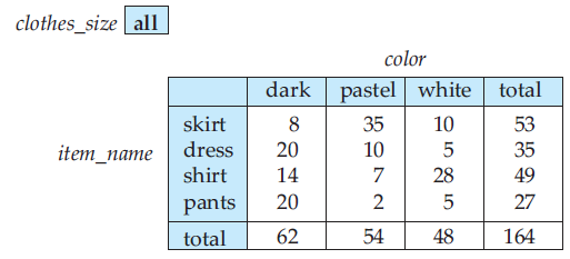 Figure 6 Cross tabulation of sales by item_name and color.
The table in Figure 6 is an example of a cross-tabulation (or cross-tab, for short), also referred to as a pivot-table. In general, a cross-tab is a table derived from a relation (say R), where values for one attribute of relation R (say A) form the row headers and values for another attributes of relation R (say B) form the column header. For example, in Figure 6, the attribute item_name corresponds to A (with values “dark”, “pastel”, and “white”), and the attribute color corresponds to to B(with attributes “skirt”, “dress”, “skirt”, and “pants”).
Each cell in the pivot-table can be identified by (ai, bj), where ai is a value for A and bj is a value for B. The values of the various cells in the pivot-table are derived from the relation R as follows: If there is at most one tuple in R with any (ai, bj) value, the value in the cell is derived from that single tuple (if any); for instance, it could be the value of one or more other attributes of the tuple. If there can be multiple tuples with an (ai, bj) value, the value in the cell must be derived by aggregation on the tuples with that value. In our example, the aggregation used is the sum of the values for attribute quantity, across all values for clothes_size, as indicated by “clothes_size: all” above the cross-tab in Figure 6. Thus, the value for cell (skirt, pastel) is 35, since there are 3 tuples in the sales that meet that criteria, with values 11, 9, 15.
In our example, the cross-tab also has an extra column and an extra row storing the totals of the cells in the row / column. Most cross-tabs have such summary rows and columns. The generalization of a cross-tab, which is two-dimensional, to n dimensions can be visualized as an n-dimensional cube, called the data cube. Figure 7 shows a data cube on the sales relation. The data cube has three dimensions, item_name, color, and clothes_size, and the measure attribute is quantity. Each cell is identified by values for these three dimensions. Each cell in the data cube contains a value, just as in a cross-tab. In Figure 7, the value contained in a cell is shown on one of the faces of the cell; other faces of the cell are shown blank if they are visible. All cells contain values, even if they are not visible. The value for a dimension may be all, in which case the cell contains a summary over all values of that dimension, as in the case of cross-tabs.
 Figure 7 Three-dimensional data cube.
The number of different ways in which the tuples can be grouped for aggregation can be large. In the example of Figure 7, there are 3 colors, 4 items, and 3 sizes resulting in a cube size of 3 × 4 × 3 = 36. Including the summary values, we obtain a 4 × 5 × 4 cube, whose size is 80. In fact, for a table with n dimensions, aggregation can be performed with grouping on each of the 2 × 2 × . . . × 2 subsets of the n dimensions.
With an OLAP system, a data analyst can look at different cross-tabs on the same data by interactively selecting the attributes in the cross-tab. Each cross-tab is a two dimensional view on a multidimensional data cube. For instance, the analyst may select a cross-tab on item_name and clothes_size or a cross-tab on color and clothes_size. The operation of changing the dimensions used in a cross-tab is called pivoting. OLAP systems allow an analyst to see a cross-tab on item_name and color for a fixed value of clothes_size, for example, large, instead of the sum across all sizes. Such an operation is referred to as slicing, since it can be thought of as viewing a slice of the data cube. The operation is sometimes called dicing, particularly when values for multiple dimensions are fixed.
When a cross-tab is used to view a multidimensional cube, the values of dimension attributes that are not part of the cross-tab are shown above the cross-tab. The value of such an attribute can be all, as shown in Figure 6, indicating that data in the cross-tab are a summary over all values for the attribute. Slicing / dicing simply consists of selecting specific values for these attributes, which are then displayed on top of the cross-tab.
OLAP systems permit users to view data at any desired level of granularity. The operation of moving from finer-granularity data to a coarser granularity (by means of aggregation) is called a rollup. In our example, starting from the data cube on the sales table, we got our example cross-tab by rolling up on the attribute clothes_size. The opposite operation—that of moving from coarser-granularity data to finer-granularity data—is called a drill down. Clearly, finer-granularity data cannot be generated from coarse-granularity data; they must be generated either from the original data, or from even finer-granularity summary data.
Analysts may wish to view a dimension at different levels of detail. For instance, an attribute of type datetime contains a date and a time of day. Using time precise to a second (or less) may not be meaningful: An analyst who is interested in rough time of day may look at only the hour value. An analyst who is interested in sales by day of the week may map the date to a day of the week and look only at that. Another analyst may be interested in aggregates over a month, or a quarter, or for an entire year.
The different levels of detail for an attribute can be organized into a hierarchy. Figure 8a shows a hierarchy on the datetime attribute. As another example, Figure 8b shows a hierarchy on location, with the city being at the bottom of the hierarchy, state above it, county at the next level, and region being the top level. In our earlier example, clothes can be grouped by category (for instance, menswear or womenswear); category would then lie above item_name in our hierarchy on clothes. At the level of actual values, skirts and dresses would fall under the womenswear category and pants and shirts under the menswear category.
 Figure 8 Hierarchies on dimensions
An analyst may be interested in viewing sales of clothes divided as menswear and womenswear, and not interested in individual values. After viewing the aggregates at the level of womenswear and menswear, an analyst may drill down the hierarchy to look at individual values. An analyst looking at the detailed level may drill up the hierarchy and look at coarser-level aggregates. Both levels can be displayed on the same cross-tab, as in Figure 9.
 Figure 9 Cross tabulation of sales with hierarchy on item_name.
3.2 Cross-Tab and Relational Tables
A cross-tab is different from relational tables usually stored in databases, since the number of columns in the cross-tab depends on the actual data. A change in the data values may result in adding more columns, which is not desirable for data storage. However, a cross-tab view is desirable for display to users. It is straightforward to represent a cross-tab without summary values in a relational form with a fixed number of columns. A cross-tab with summary rows / columns can be represented by introducing a special value all to represent subtotals, as in Figure 10. The SQL standard actually uses the null value in place of all, but to avoid confusion with regular null values, we shall continue to use all.
 Figure 10 Relational representation of the data in Figure 6.
Consider the tuples (skirt, all, all, 53) and (dress, all, all, 35). We have obtained these tuples by eliminating individual tuples with different values of color and clothes_size, and by replacing the value of quantity by an aggregate—namely, the sum of the quantities. The value all can be thought of as representing the set of all values for an attribute. Tuples with the value all for the color and clothes_size dimensions can be obtained by an aggregation on the sales relation with a group by on the column item_name. Similarly, a group by on color, clothes_size can be used to get the tuples with the value all for item_name, and a group by with no attributes (which can simply be omitted in SQL) can be used to get the tuple with value all for item_name, color, and clothes_size.
Hierarchies can also be represented by relations. For example, the fact that skirts and dresses fall under the womenswear category, and the pants and skirts under the menswear category can be represented by a relation itemcategory(item_name, category). This relation can be joined with sales relation, to get a relation that includes the category for each item. Aggregation on this joined relation allows us to get a cross-tab with hierarchy. As another example, a hierarchy on city can be represented by a single relation city_hierarchy (ID, city, state, country, region), or by multiple relations, each mapping values in one level of the hierarchy to values at the next level. We assume here that cities have unique identifiers, stored in the attribute ID, to avoid confusing between two cities with the same name, e.g., the Springfield in Missouri and the Springfield in Illinois.
3、Summary
- SQL queries can be invoked from host languages, via embedded and dynamic SQL. The ODBC and JDBC standards define application program interfaces to access SQL databases from C and Java languages programs. Increasingly, programmers use these APIs to access databases.
- Functions and procedures can be defined using SQLprocedural extensions that allow iteration and conditional (if-then-else) statements.
- Triggers define actions to be executed automatically when certain events occur and corresponding conditions are satisfied. Triggers have many uses, such as implementing business rules, audit logging, and even carrying out actions outside the database system. Although triggers were not added to the SQL standard until SQL:1999, most database systems have long implemented triggers.
- Some queries, such as transitive closure, can be expressed either by using iteration or by using recursive SQL queries. Recursion can be expressed using either recursive views or recursive with clause definitions.
- SQL supports several advanced aggregation features, including ranking and windowing queries that simplify the expression of some aggregates and allow more efficient evaluation.
- Online analytical processing (OLAP) tools help analysts view data summarized in different ways, so that can gain insight into the functioning of an organization.
- OLAP tools work on multidimensional data, characterized by dimension attributes and measure attributes.
- The data cube consists of multidimensional data summarized in different ways. Precomputing the data cube helps speed up queries on summaries of data.
- Cross-tab displays permit users to view two dimensions of multidimensional data at a time, along with summaries of the data.
- Drill down, rollup, slicing, and dicing are among the operations that uses perform with OLAP tools.
- SQL, starting with the SQL:1999 standard, provides a variety of operators for data analysis, including cube and rollup operations. Some systems support a pivot clause, which allows easy creation of cross-tabs.