
The basic structure of an SQL query consists of three clauses: select, from, and where. The query takes as its input the relations listed in the from clause, operates on them as specified in the where and select clause, and then produces a relation as the result.
1、Basic Structure of SQL Queries
We introduce the SQL syntax through examples, and describe the general structure of SQL queries later.
1.1 Queries on a Single Relation
Let us consider a simple query using our university example, “Find the names of all instructors.” Instructor names are found in the instructor relation, so we put that relation in the from clause. The instructor’s name appears in the name attribute, so we put that in the select clause.
select name from instructor;
The result is a relation consisting of a single attribute with the heading name, which is shown in Figure 1.
 Figure 1 Result of “select name from instructor“.
Now consider another query, “Find the department names of all instructors,” which can be written as:
select dept_name from instructor;
Since more than one instructor can belong to a department, a department name could appear more than once in the instructor relation. The result of the above query is a relation containing the department names, shown in Figure 2.
 Figure 2 Result of “select dept_name from instructor“.
In the formal, mathematical definition of the relational model, a relation is a set. Thus, duplicate tuples would never appear in relations. In practice, duplicate elimination is time-consuming. Therefore, SQL allows duplicate in relations as well as in the result of SQL expressions. Thus, the preceding SQL query lists each department name once for every tuple in which it appears in the instructor relation.
In those cases where we want to force the elimination of duplicates, we insert the keyword distinct after select. We can rewrite the preceding query as:
select distinct dept_name from instructor;
if we want duplicates removed. The result of the above query shown in Figure 3 would contain each department name at most once.
 Figure 3 Result of “select distinct dept_name from instructor”.
Since duplicate retention is the default, we shall not use all in our examples. To ensure the elimination of duplicates in the results of our example queries, we shall use distinct whenever it is necessary.
The select clause may also contain arithmetic expressions involving the operators + , – , * , and / operating on constants or attributes of tuples. For example, the query:
select ID, name, dept_name, salary * 1.1 from instructor;
returns a relation shown that is the same as the instructor relation, except that the attribute salary is multiplied by 1.1. Figure 4 shows what would result if we gave a 10% raise to each instructor; note, however, that it does not result in any change to the instructor relation.
 Figure 4 Result of “select ID, name, dept_name, salary * 1.1 from instructor”.
The where clause allows us to select only those rows in the result relation of the from clause that satisfy a specified predicate. Consider the query “Find the names of all instructors in the Computer Science department who have salary greater than $70000.” This query can be written in SQL as:
select name from instructor where dept_name = ‘Comp.Sci.’ and salary > 70000;
The relation that results from the preceding query is shown in Figure 5.
 Figure 5 Result of “Find the names of all instructors in the Computer Science department who have salary greater than $70000.”
SQL allows the use of the logical connectives and, or, and not in the where clause. The operands of the logical connectives can be expressions involving the comparison operators <, <=, >, >=, =, and <>. SQL allows us to use the comparison operators to compare strings and arithmetic expressions as well as special types, such as data types.
1.2 Queries on Multiple Relations
So far our example queries were on a single relation. Queries often need to access information from multiple relations. Suppose we want to answer the query “Retrieve the names of all instructors, along with their department names and department building name.”
In SQL, to answer the above query, we list the relations that need to be accessed in the from clause, and specify the matching condition in the where clause. The above query can be written in SQL as
select name, instructor.dept_name,building from instructor, department where instructor.dept_name=department.dept_name;
 Figure 6 The result of “Retrieve the names of all instructors, along with their department names and department building name.”
The naming convention requires that the relations that are present in the from clause have distinct names. This requirement causes problems in some cases, such as when information from two different tuples in the same relation needs to be combined.
We now consider the general case of SQL queries invoving multiple relations. As we have seen earlier, an SQL query can contain three types of clauses, the select clause, the from clause, and the where clause. The role of each clause is as follows:
- The select clause is used to list the attributes desired in the result of a query.
- The from clause is a list of the relations to be accessed in the evaluation of the query.
- The where clause is a predicate involving attributes of the relation in the from clause.
A typical SQL query has the form
select A1, A2, ……, An from r1, r2, ……, rm where P;
Each Ai represents an attribute, and each ri a relation. P is a predicate. If the where clause is omitted, the predicate P is true. Although the clauses must be written in the order select, from, where, the easiest way to understand the operations specified by the query is to consider the clauses in operational order: first from, then where, and then select.
The from clause by itself defines a Cartesian product of the relations listed in the clause. It is defined formally in terms of set theory, but is perhaps best understand as an iterative process that generates tuples for the result relation of the from clause.

The result relation has all attributes from all the relations in the from clause. Since the same attribute name may appear in both ri and rj, as we saw earlier, we prefix the name of the relation from which the attribute originally came, before the attribute name. For example, the relation schema for the Cartesian product of relations instructor and teaches is: (instructor.ID, name, dept_name, salary, teaches.ID, course_id, sec_id, semester, year).
 Figure 7 The Cartesian product of the instructor relation with the teaches relation.
Their Cartesian product is shown in Figure 7, which includes only a portion of the tuples that make up the Cartesian product result. The Cartesian product by itself combines tuples from instructor and teaches that are unrelated to each other. Each tuple in instructor is combined with every tuple in teaches, even those that refer to a different instructor. The result can be an extremely large relation, and it rarely makes sense to create such a Cartesian product.
Instead, the predicate in the where clause is used to restrict the combinations created by the Cartesian product to those that are meaningful for the desired answer. We would expect a query involving instructor and teaches to combine a particular tuple t in instructor with only those tuples in teaches that refer to the same instructor to which t refers. That is, we wish only to match teaches tuples with instructor tuples that have the same ID value. The following SQL query ensures this condition, and outputs the instructor name and course identifiers from such matching tuples.
select name,course_id from instructor,teaches where instructor.ID=teaches.ID;
Note that the above query outputs only instructors who have taught some course. Instructors who have not taught any course are not output. The relation that results from the preceding query is shown in Figure 8. Observe that instructors Gold, Califieri, and Singh, Who have not taught any course, do not appear in the result. Figure 8 Result of “For all instructors in the University who have taught some course, find their names and the course ID of all courses they taught.”
If we only wished to find instructor names and course identifiers for instructors in the Computer Science department, we could add an extra predicate to the where clause, as shown below.![]() Note that since the dept_name attribute occurs only in the instructor relation, we could have used just dept_name, instead of instructor.dept_name in the above query. In general, the meaning of an SQL query can be understood as follows:
Note that since the dept_name attribute occurs only in the instructor relation, we could have used just dept_name, instead of instructor.dept_name in the above query. In general, the meaning of an SQL query can be understood as follows:
⑴ Generate a Cartesian product of the relations listed in the from clause.
⑵ Apply the predicates specified in the where clause on the result of Step 1.
⑶ For each tuple in the result of Step 2, output the attributes (or results of expressions) specified in the select clause.
The above sequence of steps helps make clear what the result of an SQL query should be, not how it should be executed. A real implementation of SQL would not execute the query in this fashion; it would instead optimize evaluation by generating (as far as possible) only elements of the Cartesian product that satisfy the where clause predicates. When writing queries, you should be careful to include appropriate where clause conditions.
1.3 The Natural Join
To make the life of an SQL programmer easier for this common case, SQL supports an operation called the natural join, which we describe below. In fact SQL supports several other ways in which information from two or more relations can be joined together.
The natural join operation operates on two relations and produces a relation as the result. Unlike the Cartesian product of two relations, which concentrates each tuple of the first relation with every tuple of the second, natural join considers only those pairs of tuples with the same value on those attributes that appear in the schemas of both relations. So, going back to the example of the relations instructor and teaches, computing instructor natural join teaches considers only those pairs of tuples where both the tuple from instructor and the tuple from teaches have the same value on the common attribute, ID. Figure 9 The natural join of the instructor relation with the teaches relation.
The result relation, shown in Figure 9, has only 13 tuples, the ones that give information about an instructor and a course that that instructor actually teaches. Notice that we do not repeat those attributes that appear in the schemas of both relations; rather they appear only once. Notice also the order in which the attributes are listed: first the attributes common to the schemas of both relations, second those attributes unique to the schema of the first relation, and the finally, those attributes unique to the schema of the second relation.
Consider the query “For all instructors in the university who have taught some course, find their names and the course ID of all courses they taught”, which we wrote earlier as :
select name,course_id from instructor,teaches where instructor.ID=teaches.ID;
This query can be written more concisely using the natural-join operation in SQL as:
select name, course_id from instructor natural join teaches;
Both of the above queries generate the same result as shown below.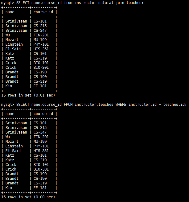
A from clause in an SQL query can have multiple relations combined using natural join, as shown here: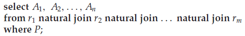 More generally, a from clause can be of the form
![]() where each Ei can be a single relation or an expression involving natural joins. For example, suppose we wish to answer the query “List the names of instructors along with the titles of courses that they teach.” T
where each Ei can be a single relation or an expression involving natural joins. For example, suppose we wish to answer the query “List the names of instructors along with the titles of courses that they teach.” T
he query can be written in SQL as follows: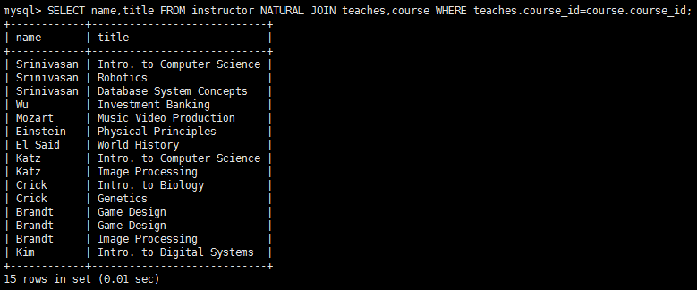 The natural join of instructor and teaches is first computed, as we saw earlier, and a Cartesian product of this result with course is computed, from which the where clause extracts only those tuples where the course identifier from the join result matches the course identifier from the course relation. Note that teaches.course_id in the where clause refers to the course_id field of the natural join result, since this field in turn came from the teaches relation.
In contrast the following SQL query does not compute the same result: To see why, note that the natural join of instructor and teaches contains the attributes (ID,name,dept_name,salary,course_id,sec_id), while the course relation contains the attributes (course_id,title,dept_name,credits). As a result, the natural join of these two would require that the dept_name attribute values from the two inputs be the same, in addition to requiring that the course_id values be the same. This query would then omit all (instructor name, course title) pairs where the instructor teaches a course in a department other than the instructor’s own department. The previous query, on the other hand, correctly outputs such pairs.
To provide the benefit of natural join while avoiding the danger of equating attributes erroneously, SQL provides a form of the natural join construct that allows you to specify exactly which columns should be equated. This feature is illustrated by the following query: The operation join … using requires a list of attribute names to be specified. Both inputs must have attributes with the specified names. Consider the operation r1 join r2 using(A1, A2). The operation is similar to r1 natural join r2, except that a pair of tuples t1 from r1 and t2 from r2 match if t1.A1 = t2.A1 and t1.A2 = t2.A2; even if r1 and r2 both have an attribute named A3, it is not required that t1.A3 = t2.A3.
Thus, in the preceding SQL query, the join construct permits teaches.dept_name and course.dept_name to differ, and the SQL query gives the correct answer.
2、Additional Basic Operations
There are number of additional basic operations that are support in SQL
2.1 The Rename Operation
Consider again the query that we used earlier: select name,course_id from instructor, teaches where instructor.ID=teaches.ID; The result of this query is a relation with the following attributes: name, course_id. The names of the attributes in the result are derived from the names of the attributes in the relations in the from clause.
We cannot, however, always derive names in this way, for several reasons: First, two relations in the from clause may have attributes with the same name, in which case an attribute name is duplicated in the result. Second, if we used an arithmetic expression in the select clause, the resultant attribute does not have a name. Third, even if an attribute name can be derived from the base relations as in the preceding example, we may want to change the attribute name in the result. Hence, SQL provides a way of renaming the attributes of a result relation. It uses the as clause, taking the form:
old-name as new-name
The as clause can appear in both the select and from clauses. For example, if we want the attribute name name to be replaced with the name instructor_name, we can rewrite the preceding query as: The as clause is particularly useful in renaming relations. One reason to rename a relation is to replace a long relation name with a shortened version that is more convenient to use elsewhere in the query. To illustrate, we rewrite the query “For all instructors in the university who have taught some course, find their names and the course ID of all courses they taught.”
 Another reason to rename a relation is a case where we wish to compare tuples in the same relation. We then need to take the Cartesian product of a relation with itself and, without renaming, it becomes impossible to distinguish one tuple from the other. Suppose that we want to write the query “Find the names of all instructors whose salary is greater than at least one instructor in the Biology department.” We can write the SQL expression:
 Observe that we could not use the notation instructor.salary, since it would not be clear which reference to instructor is intended.
In the above query, T and S can be though of as copies of the relation instructor, but more precisely, they are declared as aliases, that is as alternative names, for the relation instructor. An identifier, such as T and S, that is used to rename a relation is referred to as a correlation name in the SQL standard, but is also commonly referred to as a table alias, or a correlation variable, or a tuple variable.
2.2 String Operations
SQL specifies strings by enclosing them in single quotes, for example, ‘Computer’. A single quote character that is part of a string can be specified by using two single quote characters; for example, the string “It’s right” can be specified by “It”s right”.
The SQL standard specifies that the equality operation on string is case sensitive; as a result the expression “‘comp.sci.’=’Comp.Sci'” evaluates to false. However, some database systems, such as MySQL and SQL Server, do not distinguish uppercase from lowercase when matching strings; as a result “‘comp.sci.’=’Comp.Sci'” would evaluate to true on these databases. This default behavior can, however, be changed, either at the database level or at the level of specific attributes.
SQL also permits a variety of functions on character strings, such as concatenating (using “||”), extracting substrings, finding the length of strings, converting strings to uppercase (using the function upper(s) where s is a string) and lowercase (using the function lower(s)), removing spaces at the end of the string (using trim(s)) and so on. There are variations on the exact set of string functions supported by different database systems.
Pattern matching can be performed on strings, using the operator like. We describe patterns by using two special characters:
- Percent (%): The % character matches any substring.
- Underscore (_): The_character matches any character.
Patterns are case sensitive; that is, uppercase characters do not match lowercase characters, or vice versa. To illustrate pattern matching, we consider the following examples:
- ‘Intro%’ matches any string beginning with “Intro”.
- ‘%Comp%’ matches any string containing “Comp” as a substring, for example, ‘Intro. to Computer Science’, and ‘Computational Biology’.
- ‘___’ matches any string of exactly three characters.
- ‘___%’ matches any string of at least three characters.
SQL expresses patterns by using the like comparison operator. Consider the query “Find the names of all department whose building name includes the substring ‘Watson’.” This query can be written as: For patterns to include the special pattern character (that is, % and_), SQL allows the specification of an escape character. The escape character is used immediately before a special pattern character to indicate that the special pattern character is to be treated like a normal character. We define the escape character for a like comparison using the escape keyword. To illustrate, consider the following patterns, which use a backslash ( \ ) as the escape character:
- like ‘ab\%cd%’ escape ‘ \ ‘ matches all strings beginning with “ab%cd”.
- like ‘ab\\cd%’ escape ‘ \ ‘ matches all string beginning with “ab\cd”.
SQL allows us to search for mismatches instead of matches by using the not like comparison operator. Some databases provide variants of the like operation which do not distinguish lower and upper case.
SQL:1999 also offers a similar to operation, which provides more powerful pattern matching than the like operation; the syntax for specifying patterns is similar to that used in Unix regular expressions.
2.3 Attribute Specification in Select Clause
The asterisk symbol ” * ” can be used in the select clause to denote “all attributes.” Thus, the use of instructor.* in the select clause of the query: indicates that all attributes of instructor are to be selected. A select clause of the form select * indicates that all attributes of the result relation of the from clause are selected.
2.4 Ordering the Display of Tuples
SQL offers the user some control over the order in which tuples in a relation are displayed. The order by clause causes the tuples in the result of a query to appear in sorted order. To list in alphabetic order all instructors in the Physics department, we write: By default, the order by clause lists items in ascending order. To specify the sort order, we may specify desc for descending order or asc for ascending order. Furthermore, ordering can be performed on multiple attributes. Suppose that we wish to list the entire instructor relation in descending order of salary. If several instructors have the same salary, we order them in ascending order by name. We express this query in SQL as follows:
2.5 Where Clause Predicates
SQL includes a between comparison operator to simplify where clauses that specify that a value be less than or equal to some value and greater than or equal to some other value. If we wish to find the names of instructors with salary amounts between $90000 and $100000, we can use the between comparison to write: instead of:
 Similarly, we can use the not between comparison operator.
We can extend the preceding query that finds instructor names along with course identifiers, which we saw earlier, and consider a more complicated case in which we require also that the instructors be from the Biology department: “Find the instructor names and the courses they taught for all instructors in the Biology department who have taught some course.” To write this query, we can modify either of the SQL queries we saw earlier, by adding an extra condition in the where clause. We show below the modified form of the SQL query that does not use natural join. SQL permits us to use the notation ( v1, v2, … , vn ) to denote a tuple of arity n containing values v1, v2, … , vn. The comparison operators can be used on tuples, and the ordering is defined lexicographically. For example, (a1, a2) <= (b1, b2) is true if a1 <= b1, and a2 <= b2; similarly, the two tuples are equal if all their attributes are equal. Thus, the preceding SQL query can be rewritten as follows: