
Linked lists bring us into a world of computing that is markedly different from that of arrays and structures. With arrays and structures, we save an item in memory and later refer to it by name (or by index) in much the same manner as we might put a piece of information in a file drawer or an address book; with linked lists, the manner in which we save information makes it more difficult to access but easier to rearrange. Working with data that are organized in linked lists is called list processing.When we use arrays, we are susceptible to program bugs involving out-of-bounds array accesses. The most common bug that we encounter when using linked lists is a similar bug where we reference an undefined pointer. Another common mistake is to use a pointer that we have changed unknowingly. One reason that this problem arises is that we may have multiple pointers to the same node without necessarily realizing that that is the case. Program 1 in Elementary Data Structures ~ Linked Lists I avoids several such problems by using a circular list that is never empty, so that each link always refers to a well-defined node, and each link can also be interpreted as referring to the list.
Developing correct and efficient code for list-processing applications is an acquired programming skill that requires practice and patience to develop.
Definition 1 A linked list is either a null link or a link to a node that contains an item and a link to a linked list.
This definition is more restrictive than Definition previous, but it corresponds more closely to the mental model that we have when we write list-processing code. Rather than exclude all the other various conventions by using only this definition, and rather than provide specific definitions corresponding to each convention, we let both stand, with the understanding that it will be clear from the context which type of linked list we are using.
One of the most common operations that we perform on lists is to traverse them: We scan through the items on the list sequentially, performing some operation on each. For example, if x is a pointer to the first node of a list, the final node has a null pointer, and visit is a function that takes an item as an argument, then we might write![]() to traverse the list. This loop (or its equivalent while form) is as ubiquitous in list-processing programs as is in the corresponding
to traverse the list. This loop (or its equivalent while form) is as ubiquitous in list-processing programs as is in the corresponding![]() in array-processing programs.
in array-processing programs.
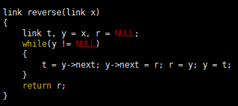
Program 1 is an implementation of a simple list-processing task, reversing the order of the nodes on a list. It takes a linked list as an argument, and returns a linked list comprising the same nodes, but with the order reversed. Figure 1 shows the change that the function makes for each node in its main loop. Such a diagram makes it easier for us to check each statement of the program to be sure that the code changes the links as intended, and programmers typically use these diagrams to understand the operation of list-processing implementations.
Program 1 List reversal
This function reverses the links in a list, returning a pointer to the final node, which then points to the next-to-final node, and so forth, with the link in the first node of the original list set to NULL. To accomplish this task, we need to maintain links to three consecutive nodes in the list.

Figure 1 List reversal
To reverse the order of a list, we maintain a pointer r to the portion of the list already processed, and a pointer y to the portion of the list not yet seen. This diagram shows how the pointers change for each node in the list. We save a pointer to the node following y in t, change y’s link to point to r, and then move r to y and y to t.
Figure 1 shows the change that the function makes for each node in its main loop. Such a diagram makes it easier for us to check each statement of the program to be sure that the code changes the links as intended, and programmers typically use these diagrams to understand the operation of list-processing implementations.
Program 2 is an implementation of another list-processing task: rearranging the nodes of a list to put their items in sorted order. It generates N random integers, puts them into a list in the order that they were generated, rearranges the nodes to put their items in sorted order, and prints out the sorted sequence. The expected running time of this program is proportional to N², so the program is not useful for large N.
 Program 2 List insertion sort
This code generates N random integers between 0 and 999, builds a linked list with one number per node (first for loop), and then rearranges the nodes so that the numbers appear in order when we traverse the list (second for loop). To accomplish the sort, we maintain two lists, an input (unsorted) list and an output (sorted) list. On each iteration of the loop, we remove a node from the input and insert it into position in the output. The code is simplified by the use of head nodes for each list, that contain the links to the first nodes on the lists.

The list in Program 2 illustrate another commonly used convention: We maintain a dummy node called a head node at the beginning of each list. We ignore the item field in a list’s head node, but maintain its link as the pointer to the node containing the first item in the list. The program uses two lists: one to collect the random input in the first loop, and the other to collect the sorted output in the second loop. Figure 2 diagrams the changes that Program 2 makes during one iteration of its main loop. We take the next node off the input list, find where it belongs in the output list, and link it into position.
 Figure 2 Linked-list sort
This diagram depicts one step in transforming an unordered linked list (pointed to by a) into an ordered one (pointed to by b), using insertion sort. We take the first node of the unordered list, keeping a pointer to it in t (top). Then, we search through b to find the first node x with x->next->item > t->item (or x->next = NULL), and insert t into the list following x (center). These operations reduce the length of a by one node, and increase the length of b by one node, keeping b in order (bottom). Iterating, we eventually exhaust a and have the nodes in order in b.
The primary reason to use the head node at the beginning becomes clear when we consider the process of adding the first node to the sorted list. This node is the one in the input list with the smallest item, and it could be anywhere on the list. We have three options:
- Duplicate the for loop that finds the smallest item and set up a one-node list in the same manner as in Josephus problem.
- Test whether the output list is empty every time that we wish to insert a node.
- Use a dummy head node whose link points to the first node on the list, as in the given implementation
The first option inelegant and requires extra code; the second is also inelegant and requires extra time.
The use of a head node does incur some cost (the extra node), and we can avoid the head node in many common applications. There are no hard-and fast rules about whether or not to use dummy nodes——the choice is a matter of style combined with an understanding of effects on performance. Good programmers enjoy the challenge of picking the convention that most simplifies the task at hand.

Table 1 Head and tail conventions in linked lists
This table gives implementations of basic list-processing operations with five commonly used conventions. This type of code is used in simple applications where the list-processing code is inline.
For reference, a number of options for linked-list conventions are laid out in Table 1. In all the cases in Table 1, we use a pointer head to refer to the list, and we maintain a consistent stance that our program manages links to nodes, using the given code for various operations. Allocating and freeing memory for nodes and filling them with information is the same for all the conventions. Robust functions implementing the same operations would have extra code to check for error conditions. The purpose of the table is to expose similarities and differences among the various options.
Another important situation in which it is sometimes convenient to use head nodes occurs when we want to pass pointers to lists as arguments to functions that may modify the list, in the same way that we do for arrays. Using a head node allows the function to accept or return an empty list. If we do not have a head node, we need a mechanism for the function to inform the calling program when it leaves an empty list. One such mechanism—the one used for the function in Program 1—is to have list-processing functions take pointers to input lists as arguments and return pointers to output lists. With this convention, we do not need to use head nodes. Furthermore, it is well suited to recursive list processing.
 Program 3 List-processing interface
This code, which might be kept in an interface file list.h, specifies the types of nodes and links, and declares some of the operations that we might want to perform on them. We declare our own functions for allocating and freeing memory for list nodes. The function initNodes is for the convenience of the implementation. The typedef for Node and the functions Next and Item allow clients to use lists without dependence upon implementation details.
Program 3 illustrates declarations for a set of black-box functions that implement the basic list operations, in case we choose not to repeat the code inline. Program 4 is our Josephus-election program recast as a client program that uses this interface. Identifying the important operations that we use in a computation and defining them in an interface gives us the flexibility to consider different concrete implementations of critical operations and to test their effectiveness. We consider one implementation for the operations defined in Program 3 in Program 5, but we could also try other alternatives without changing Program 4 at all.
 Program 4 List allocation for the Josephus problem
This program for the Josephus problem is an example of a client program utilizing the list-processing primitives declared in Program 3 and implemented in Program 5.
By adding more links, we can add the capability to move backward through a linked list. For example, we can support the operation “find the item before a given item” by using a doubly linked list in which we maintain two links for each node: one (prev) to the item before, and another (next) to the item after. With dummy nodes or a circular list, we can ensure that x, x->next->prev, and x->prev->next are the same for every node in a doubly linked list.
 Figure 3 Deletion in a doubly-linked list
In a doubly-linked list, a pointer to a node is sufficient information for us to be able to remove it, as diagrammed here. Given t, we set t->next->prev to t->prev (center) and t->prev->next to t->next (bottom).
 Figure 4 Insertion in a doubly-linked list
To insert a node into a doubly-linked list, we need to set four pointers. We can insert a new node after a given node (diagrammed here) or before a given node. We insert a given node t after another given node x by setting t->next to x->next and x->next->prev to t (center), and then setting x->next to t and t->prev to x (bottom).
Figure 3 and 4 show the basic link manipulations required to implement delete, insert after, and insert before, in a doubly linked list. Note that, for delete, we do not need extra information about the node before it (or the node after it) in the list, as we did for singly linked lists—that information is contained in the node itself.
Indeed, the primary significance of doubly linked lists is that they allow us to delete a node when the only information that we have about the node is a link to it. Typical situations are when the link is passed as an argument in a function call, and when the node has other links and is also part of some other data structure. Providing this extra capability doubles the space needed for links in each node and doubles the number of link manipulations per basic operation, so doubly linked lists are not normally used unless specifically called for.
Linked lists are many programmers’ first exposure to an abstract data structure that is under the programmers’ direct control. They represent an essential tool for our use in developing the high-level abstract data structures that we need for a host of important problems, as we shall see.
An advantage of linked lists over arrays is that linked lists gracefully grow and shrink during their lifetime. In particular, their maximum size does not need to be known in advance. One important practical ramification of this observation is that we can have several data structures share the same space, without paying particular attention to their relative size at any time.
The crux of the matter is to consider how the system function malloc might be implemented. For example, when we delete a node from a list, it is one thing for us to rearrange the links so that the node is no longer hooked into the list, but what does the system do with the space that the node occupied? And how does the system recycle space such that it can always find space for a node when malloc is called and more space is needed? The mechanisms behind these questions provide another example of the utility of elementary list processing.
The system function free is the counterpart to malloc. When we are done using a chunk of allocated memory, we call free to inform the system that the chunk is available for later use. Dynamic memory allocation is the process of managing memory and responding to calls on malloc and free from client programs.
When we are calling malloc directly in applications such as Program 2, all the calls request memory blocks of the same size. This case is typical, and an alternate method of keeping track of memory available for allocation immediately suggests itself: Simply use a linked list! All nodes that are not on any list that is in use can be kept together on a single linked list. We refer to this list as the free list. When we need to allocate space for a node, we get it by deleting it from the free list; when we remove a node from any of our lists, we dispose of it by inserting it onto the free list.
 Program 5 Implementation of list-processing interface
This program gives implementations of the functions declared in Program 3, and illustrates a standard approach to allocating memory for fixed-size nodes. We build a free list that is initialized to the maximum number of nodes that our program will use, all linked together. Then, when a client program allocates a node, we remove that node from the free list; when a client program frees a node, we link that node in to the free list.
By convention, client programs do not refer to list nodes except through functions calls, and nodes returned to client programs have self-links. These conventions provide some measure of protection against referencing undefined pointers.
Program 5 is an implementation of the interface defined in Program 3, including the memory-allocation functions. When compiled with Program 4, it produces the same result as the direct implementation with which we began in Program 1 in Elementary Data Structures ~ Linked Lists I .
![]()
Maintaining the free list for fixed-size nodes is a trivial task, given the basic operations for inserting nodes onto and deleting nodes from a list.
 Figure 5 Array representation of a linked list, with free list
This version of Figure 4 in Elementary Data Structures ~ Linked Lists I shows the result of maintaining a free list with the nodes deleted from the circular list, with the index of first node on the free list given at the left. At the end of the process, the free list is a linked list containing all the items that were deleted. Following the links, starting at 1, we see the items in the order 2 9 6 3 4 7 1 5, which is the reverse of the order in which they were deleted.
Figure 5 illustrates how the free list grows as nodes are freed, for Program 4. For simplicity, the figure assumes a linked-list implementation (no head node) based on array indices.
Implementing a general-purpose memory allocator in a C environment is much more complex than is suggested by our simple examples, and the implementation of malloc in the standard library is certainly not as simple as is indicated by Program 5. One primary difference between the two is that malloc has to handle storage-allocation requests for nodes of varying sizes, ranging from tiny to huge. Several clever algorithms have been developed for this purpose. Another approach that is used by some modern systems is to relieve the user of the need to free nodes explicitly by using garbage-collection algorithms to remove automatically any nodes not referenced by any link. Several clever storage management algorithms have also been developed along these lines. We will not consider them in further detail because their performance characteristics are dependent on properties of specific systems and machines.
Programs that can take advantages of specialized knowledge about an application often are more efficient than general-purpose programs for the same task. Memory allocation is no exception to this maxim. An algorithm that has to handle storage requests of varying sizes cannot know that we are always going to be making requests for blocks of one fixed size, and therefore cannot take advantage of that fact. Paradoxically, another reason to avoid general-purpose library functions is that doing so makes programs more portable—we can protect ourselves against unexpected performance changes when the library changes or when we move to a different system. Many programmers have found that using a simple memory allocator like the one illustrated in Program 5 is an effective way to develop efficient and portable programs that use linked lists. This approach applies to a number of the algorithms that we will consider throughout the series, which make similar kinds of demands on the memory-management system.