
Selection sort, insertion sort, and bubble sort are all quadratic-time algorithms both in the worst and in the average case, and none requires extra memory. Their running times thus differ by only a constant factor, but they operate quite differently, as illustrated in Figures 1 through 3.
1、Performance Characteristics of Elementary Sorts
Generally, the running time of a sorting algorithm is proportional to the number of comparisons that the algorithm uses, to the number of times that items are moved or exchanged, or to both. For random input, comparing the methods involves studying constant-factor differences in the numbers of comparisons and exchanges and constant-factor differences in the lengths of the inner loops. For input with special characteristics, the running times of the methods may differ by more than a constant factor. In this section, we look closely at the analytic results in support of this conclusion.
 Figure 1 Dynamic characteristics of insertion and selection sorts
These snapshots of insertion sort (left) and selection sort (right) in action on a random permutation illustrate how each method progresses through the sort. We represent an array being sorted by plotting i vs. a[ i ] for each i. Before the sort, the plot is uniformly random; after the sort, it is a diagonal line from bottom left to top right. Insertion sort never looks ahead of its current position in the array; selection sort never looks back. Figure 2 Comparisons and exchanges in elementary sorts
This diagram highlights the differences in the way that insertion sort, selection sort, and bubble sort bring a file into order. The file to be sorted is represented by lines that are to be sorted according to their angles. Black lines correspond to the items accessed during each pass of the sort; gray lines correspond to items no touched. For insertion sort (left), the element to be inserted goes about halfway back through the sorted part of the file on each pass. Selection sort (center) and bubble sort (right) both go through the entire unsorted part of the array to find the next smallest element there for each pass; the difference between the methods is that bubble sort exchanges any adjacent out-of-order elements that it encounters, whereas selection sort just exchanges the minimum into position. The effect of this difference is that the unsorted part of the array becomes more nearly sorted as bubble sort progresses. Figure 3 Dynamic characteristics of two bubble sorts
Standard bubble sort (left) operates in a manner similar to selection sort in that each pass brings one element into position, but it also brings some order into other parts of the array, in an asymmetric manner. Changing the scan through the array to alternate between beginning to end and end to beginning gives a version of bubble sort called shaker sort (right), which finishes more quickly.
Property 1 Selection sort uses about N²/2 comparisons and N exchanges.
We can verify this property easily by examining the sample run in Figure 2 in Sorting~Elementary Sorting Methods I, which is an N-by-N table in which unshaded letters correspond to comparisons. About one-half of the elements in the table are unshaded——those above the diagonal. The N – 1 (not the final one) elements on the diagonal each correspond to an exchange. More precisely, examination of the code reveals that, for each i from 1 to N – 1, there is one exchange and N – i comparisons, so there is a total of N – 1 exchanges and (N – 1) + (N – 2) + · · · + 2 + 1 = N (N – 1) / 2 comparisons. These observations hold no matter what the input data are; the only part of selection sort that does depend on the input is the number of times that min is updated. In the worst case, this quantity could also be quadratic; in the average, however, it is just O(N log N) (see reference section), so we can expect the running time of selection sort to be insensitive to the input.
Property 2 Insertion sort uses about N² / 4 comparisons and N² / 4 half-exchanges (moves) on the average, and twice that many at worst.
As implemented in Program 3 in Sorting~Elementary Sorting Methods I, the number of comparisons and of moves is the same. Just as for Property 1, this quantity is easy to visualize in the N-by-N diagram in Figure 3 in Sorting~Elementary Sorting Methods I that gives the details of the operation of the algorithm. Here, the elements below the diagonal are counted——all of them, in the worst case. For random input, we expect each element to go about halfway back, on the average, so one-half of the elements below the diagonal should be counted.
Property 3 Bubble sort uses about N² / 2 comparisons and N² / 2 exchanges on the average and in the worst case.
The i th bubble sort pass requires N – i compare-exchange operations, so the proof goes as for selection sort. When the algorithm is modified to terminate when it discovers that the file is sorted, the running time depends on the input. Just one pass is required if the file is already in order, but the i the pass requires N – i comparisons and exchanges if the file is in reverse order. The average-case performance is not significantly better than the worst case, as stated, although the analysis that demonstrates this fact is complicated (see reference section).
Although the concept of a partially sorted file is necessarily rather imprecise, insertion sort and bubble sort work well for certain types of nonrandom files that often arise in practice. General-purpose sorts are commonly misused for such applications. For example, consider the operation of insertion sort on a file that is already sorted. Each element is immediately determined to be in its proper place in the file, and the total running time is linear. The same is true for bubble sort, but selection sort is still quadratic.
Definition 1 An inversion is a pair of keys that are out of order in the file.
To count the number of inversions in a file, we can add up, for each element, the number of elements to its left that are greater (we refer to this quantity as the number of inversions corresponding to the element). But this count is precisely the distance that the elements have to move when inserted into the file during insertion sort. A file that has some order will have fewer inversions than will one that is arbitrarily scrambled.
In one type of partially sorted file, each item is close to its final position in the file. For example, some people sort their hand in a card game by first organizing the cards by suit, to put their cards close to their final position, then considering the cards one by one. We shall be considering a number of sorting methods that word in much the same way——they bring elements close to final positions in early stages to produce a partially sorted file with every element not far from where it ultimately must go. Insertion sort and bubble sort (but not selection sort) are efficient methods for sorting such files.
Property 4 Insertion sort and bubble sort use a linear number of comparisons and exchanges for files with at most a constant number of inversions corresponding to each element.
As just mentioned, the running time of insertion sort is directly proportional to the number of inversions in the file. For bubble sort (here, we are referring to Program 4 in Sorting~Elementary Sorting Methods I, modified to terminate when the file is sorted), the proof is more subtle. Each bubble sort pass reduces the number of smaller elements to the right of any element by precisely 1 (unless the number was already 0), so bubble sort uses at most a constant number of passes for the types of files under consideration, and therefore does at most a linear number of comparisons and exchanges.
In another type of partially sorted file, we perhaps have appended a few elements to a sorted file or have edited a few elements in a sorted file to change their keys. This kind of file is prevalent in sorting applications. Insertion sort is an efficient method for such files; bubble sort and selection sort are not.
Property 5 Insertion sort uses a linear number of comparisons and exchanges for files with at most a constant number of elements having more than a constant number of corresponding inversions.
Table 1 Empirical study of elementary sorting algorithms
Insertion sort and selection sort are about twice as fast as bubble sort for small files, but running times grow quadratically (when the file size grows by a factor of 2, the running time grows by a factor of 4). None of the methods are useful for large randomly ordered files——for example, the numbers corresponding to those in this table are less than 2 for the shellsort algorithms in later section. When comparisons are expensive——for example, when the keys are strings——then insertion sort is much faster than the other two because it uses many fewer comparisons. Not included here is the case where exchanges are expensive; then selection sort is best. Key:
Key:
S Selection sort (Program 2 in Sorting~Elementary Sorting Methods I);
I* Insertion sort, exchange-based (Program 1 in Sorting~Elementary Sorting Methods I);
I Insertion sort (Program 3 in Sorting~Elementary Sorting Methods I);
B Bubble sort (Program 4 in Sorting~Elementary Sorting Methods I);
B* Shaker sort;
The running time of insertion sort depends on the total number of inversions in the file, and does not depend on the way in which the inversions are distributed.
To draw conclusions about running time from Properties 1 through 5, we need to analyze the relative cost of comparisons and exchanges, a factor that in turn depends on the size of the items and keys (see Table 1). For example, if the items are one-word keys, then are exchange (four array accesses) should be about twice as expensive as a comparison. In such a situation, the running times of selection and insertion sort are roughly comparable, but bubble sort is slower. But if the items are large in comparison to the keys, then selection sort will be be best.
Property 6 Selection sort runs in linear time for files with large items and small keys.
Let M be the ratio of the size of the item to the size of the key. Then we can assume the cost of a comparison to be 1 time unit and the cost of an exchange to be M time units. Selection sort takes about N² / 2 time units for comparisons and about N M time units for exchanges. If M is larger than a constant multiple of N, then the N M term dominates the N² term, so the running time is proportional to N M, which is proportional to the amount of time that would be required to move all the data.
For example, if we have to sort 1000 items that consist of 1-word keys and 1000 words of data each, and we actually have to rearrange the items, then we cannot do better than selection sort, since the running time will be dominated by the cost of moving all 1 million words of data. In later Section, we shall see alternatives to rearranging the data.
2、Shellsort
Insertion sort is slow because the only exchanges it does involve adjacent items, so items can move through the array only one place at a time. For example, if the item with the smallest key happens to be at the end of the array, N steps are needed to get it where it belongs. Shellsort is a simple extension of insertion sort that gains speed by allowing exchanges of elements that are far apart.
The idea is to rearrange the file to give it the property that taking every h th element (starting anywhere) yields a sorted file. Such a file is said to be h-sorted. Put another way, an h-sorted file is h independent sorted files, interleaved together. By h-sorting for some large values of h, we can move elements in the array long distances and thus make it easier to h-sort for smaller values of h. Using such a procedure for any sequence of values of h that ends in 1 will produce a sorted file: that is the essence of shellsort.
One way to implement shellsort would be, for each h, to use insertion sort independently on each of the h subfiles. Despite the apparent simplicity of this process, we can use an even simpler approach, precisely because the subfiles are independent. When h-sorting the file, we simply insert it among the previous elements in its h-subfile by moving larger elements to the right (see Figure 4). We accomplish this task by using the insertion-sort code, but modified to increment or decrement by h instead of 1 when moving through the file. This observation reduces the shellsort implementation to nothing more than an insertion-sort-like pass through the file for each increment, as in Program 1. The operation of this program is illustrated in Figure 5.
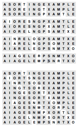 Figure 4 Interleaving 4-sorts
The top part of this diagram shows the process of 4-sorting a file of 15 elements by first insertion sorting the subfile at positions 0, 4, 8, 12, then insertion sorting the subfile at positions 1, 5, 9, 13, then insertion sorting the subfile at positions 2, 6, 10, 14, then insertion sorting the subfile at positions 3, 7, 11. But the four subfiles are independent, so we can achieve the same result by inserting each element into position into its subfile, going back four at a time (bottom). Taking the first row in each section of the top diagram, then the second row in each section, and so forth, gives the bottom diagram.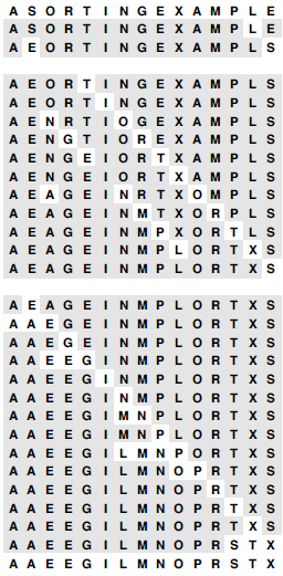 Figure 5 Shellsort example
Sorting a file by 13-sorting (top), then 4-sorting (center), then 1-sorting (bottom) does not involve many comparisons (as indicated by the unshaded elements). The final pass is just insertion sort, but no element has to move far because of the order in the file due to the first two passes.
How do we decide what increment sequence to use? In general, this question is a difficult one to answer. Properties of many different increment sequences have been studied in the literature, and some have been found that work well in practice, but no provably best sequence has been found. In practice, we generally use sequences that decrease roughly geometrically, so the number of increments is logarithmic in the size of the file. For example, if each increment is about one-half of the previous, then we need only about 20 increments to sort a file of 1 million elements; if the ratio is about one-quarter, then 10 increments will suffice. Using as few increments as possible is an important consideration that is easy to respect——we also need to consider arithmetical interactions among the increments such as the size of their common divisors and other properties.
The practical effect of finding a good increment sequence is limited to perhaps a 25% speedup, but the problem presents an intriguing puzzle that provides a good example of the inherent complexity in an apparently simple algorithm. The increment sequence 1 4 13 40 121 364 1093 3280 9841 . . . that is used in Program 1, with a ratio between increments of about one-third, was recommended by Knuth in 1969. It is easy to compute (start with 1, generate the next increment by multiplying by 3 and adding 1) and leads to a relatively efficient sort, even for moderately large files, as illustrated in Figure 6.
Many other increment sequences lead to a more efficient sort but it is difficult to beat the sequence in Program 1 by more than 20% even for relatively large N. One increment sequence that does so is 1 8 23 77 281 1073 4193 16577 . . . , the sequence ![]() which has provably faster worst-case behavior (see Property 10). Figure 8 shows that this sequence and Knuth’s sequence ——and many other sequences——have similar dynamic characteristics for large files. The possibility that even better increment sequences exist is still real. A few ideas on improved increment sequences are explored in the exercises.
which has provably faster worst-case behavior (see Property 10). Figure 8 shows that this sequence and Knuth’s sequence ——and many other sequences——have similar dynamic characteristics for large files. The possibility that even better increment sequences exist is still real. A few ideas on improved increment sequences are explored in the exercises.
Program 1 Shellsort
If we do not use sentinels and then replace every occurrence of “1” by “h” in insertion sort, the resulting program h-sorts the file. Adding an outer loop to change the increments leads to this compact shellsort implementation, which uses the increment sequence 1 4 13 40 121 364 1093 3280 9841 . . . .
![]()
Figure 6 Shellsorting a random permutation
The effect of each of the passes in Shellsort is to bring the file as a whole closer to sorted order. The file is first 40-sorted, then 13-sorted, then 4-sorted, then 1-sorted. Each pass brings the file closer to sorted order.

On the other hand, there are some bad increment sequences: for example 1 2 4 8 16 32 64 128 256 512 1024 2048 . . . (the original sequence suggested by Shell when he proposed the algorithm in 1959) is likely to lead to bad performance because elements in odd positions are not compared against elements in even positions until the final pass. The effect is noticeable for random files, and is catastrophic in the worst case: The method degenerates to require quadratic running time if, for example, the half of the elements with the smallest values are in even positions and the half of the elements with the largest values are in the odd positions.
Program 1 computes the next increment by dividing the current one by 3, after initializing to ensure that the same sequence is always used. Another option is just to start with h = N / 3 or with some other function of N. It is best to avoid such strategies, because bad sequences of the type described in the previous paragraph are likely to turn up for some values of N.
Our description of the efficiency of shellsort is necessarily imprecise, because no one has been able to analyze the algorithm. This gap in our knowledge makes it difficult not only to evaluate different increment sequences, but also to compare shellsort with other methods analytically. Not even the functional form of the running time for shellsort is known (furthermore, the form depends on the increment sequence). Knuth found that the functional forms N(log N)² and N × N¼ both fit the data reasonably well, and later research suggests that a more complicated function of the form![]() is involved for some sequences. We conclude this section by digressing into a discussion of several facts about the analysis of shellsort that are known. Our primary purpose in doing so is to illustrate that even algorithms that are apparently simple can have complex properties, and that the analysis of algorithms is not just of practical importance but also can be intellectually challenging. Readers intrigued by the idea of finding a new and improved shellsort increment sequence may find the information that follows useful; other readers may wish to skip to later section.
is involved for some sequences. We conclude this section by digressing into a discussion of several facts about the analysis of shellsort that are known. Our primary purpose in doing so is to illustrate that even algorithms that are apparently simple can have complex properties, and that the analysis of algorithms is not just of practical importance but also can be intellectually challenging. Readers intrigued by the idea of finding a new and improved shellsort increment sequence may find the information that follows useful; other readers may wish to skip to later section.
Property 7 The result of h-sorting a file that is k-ordered is a file that is both h- and k-ordered.
This fact seems obvious, but is tricky to prove.
Property 8 Shellsort does less than N(h-1)(k-1)/g comparisons to g-sort a file that is h- and k-ordered, provided that h and k are relatively prime.
The basis for this fact is illustrated in Figure 7. No element farther than (h-1)(k-1) positions to the left of any given element x can be greater than x, if h and k are relatively prime. When g-sorting, we examine at most one out of every g of those elements.
Property 9 Shellsort does less than O(N×N½) comparisons for the increments 1 4 13 40 121 364 1093 3280 9841 . . . .
For large increments, there are h subfiles of size about N/h, for a worst-case cost about N² / h. For small increments, Property 8 implies that the cost is about Nh. The result follows if we use the better of these bounds for each increment. It holds for any relatively prime sequence that grows exponentially.
Property 10 Shellsort does less than O(N×N⅓) comparisons for the increments 1 8 23 77 281 1073 4193 16577 . . . .
The proof of this property is along the lines of the proof of Property 9. The property analogous to Property 8 implies that the cost for small increments is about N×h½. Proof of this property requires number theory that is beyond the scope of this series. The increment sequences that we have discussed to this point are effective because successive elements are relatively prime. Another family of increment sequences is effective precisely because successive elements are not relatively prime.
 Figure 7 A 4- and 13- ordered file.
The bottom row depicts an array, with shaded boxes depicting those items that must be smaller than or equal to the item at the far right, if the array is both 4- and 13-ordered. The four rows at top depict the origin of the pattern. If the item at right is at array position i, the 4-ordering means that items at array positions i – 4, i – 8, i – 12, . . . are smaller or equal (top); 13-ordering means that the item at i – 13, and, therefore, because of 4-ordering, the items at i – 17, i – 21, i – 25, . . . are smaller or equal (second from top); also, the item at i – 26, and, therefore, because of 4-ordering, the items at i – 30, i – 34, i – 38, . . . are smaller or equal (third from top); and so forth. The white squares remaining are those that could be larger than the item at left; there are at most 18 such items (and the one that is farthest away is at i – 36). Thus, at most 18N comparisons are required for an insertion sort of a 13-ordered and 4-ordered file of size N.
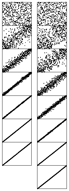 Figure 8 Dynamic characteristics of shellsort (two different increment sequences)
In this representation of shellsort in operation, it appears as though a rubber band, anchored at the corners, is pulling the points toward the diagonal. Two increment sequences are depicted: 121 40 13 4 1 (left) and 209 109 41 19 5 1 (right). The second requires one more pass than the first, but is faster because each pass is more efficient.
In particular, the proof of Property 8 implies that, in a file that is 2-ordered and 3-ordered, each element moves at most one position during the final insertion sort. That is, such a file can be sorted with one bubble-sort pass (the extra loop in insertion sort is not needed). Now, if a file is 4-ordered and 6-ordered, then it also follows that each elements moves at most one position when we are 2-sorting it (because each subfile is 2-ordered and 3-ordered); and if a file is 6-ordered and 9-ordered, each element moves at most one position when we are 3-sorting it. Continuing this line of reasoning, we are led to the following idea, which was developed by Pratt in 1971.
Property 11 Shellsort does less than O(N (log N)²) comparisons for the increments 1 2 3 4 6 9 8 12 18 27 16 24 36 54 81 . . . .
Consider the following triangle of increments, where each number in the triangle is two times the number above and to the right of it and also three times the number above and to the left of it.
If we use these numbers from bottom to top and right to left as a shellsort increment sequence, then every increment x after the bottom row is preceded by 2x and 3x, so every subfile is 2-ordered and 3-ordered, and no element moves more than one position during the entire sort! The number of increments in the triangle that are less than N is certainly less than (log2N)².
Pratt’s increments tend not to work as well as the others in practice, because there are too many of them. We can use the same principle to build an increment sequence from any two relatively prime numbers h and k. Such sequences do well in practice because the worst-case bounds corresponding to Property 11 overestimate the cost for random files. The problem of designing good increment sequences for shellsort provides an excellent example of the complex behavior of a simple algorithm. We certainly will not be able to focus at this level of detail on all the algorithms that we encounter (not only do we not have the space, but also, as we did with shellsort, we might encounter mathematical analysis beyond the scope of this series, or even open research problems). However, many of the algorithms in this series are the product of extensive analytic and empirical studies by many researchers over the past several decades, and we can benefit from this work. This research illustrates that the quest for improved performance can be both intellectually challenging and practically rewarding, even for simple algorithms. Table 2 gives empirical results that show that several approaches to designing increment sequences work well in practice; the relatively short sequence 1 8 23 77 281 1073 4193 16577 . . . is among the simplest to use in a shellsort implementation.
Figure 9 shows that shellsort performs reasonably well on a variety of kinds of files, rather than just on random ones. Indeed, constructing a file for which shellsort runs slowly for a given increment sequence is a challenging exercise. As we have mentioned, there are some bad increment sequences for which shellsort may require a quadratic number of comparisons in the worst case, but much lower bounds have been shown to hold for a wide variety of sequences.
Table 2 Empirical study of shellsort increment sequences
Shellsort is many times faster than the other elementary methods even when the increments are powers of 2, but some increment sequences can speed it up by another factor of 5 or more. The three best sequences in this table are totally difference in design. Shellsort is a practical method even for large files, particularly by contrast with selection sort, insertion sort, and bubble sort (see Table 1). Key:
Key:
O 1 2 4 8 16 32 64 128 256 512 1024 2048 . . .
K 1 4 13 40 121 364 1093 3280 9841 . . . (Property 9)
G 1 2 4 10 23 51 113 249 548 1207 2655 5843 . . .
S 1 8 23 77 281 1073 4193 16577 . . . (Property 10)
P 1 7 8 49 56 64 343 392 448 512 2401 2744 . . .
I 1 5 19 41 109 209 505 929 2161 3905 . . .
Figure 9 Dynamic characteristics of shellsort for various types of files
These diagrams show shellsort, with the increments 209 109 41 19 5 1, in operation on files that are random, Gaussian, nearly ordered, nearly reverse-ordered, and randomly ordered with 10 distinct key values (left to right, on the top). The running time for each pass depends on how well ordered the file is when the pass begins. After a few passes, these files are similarly ordered; thus, the running time is not particularly sensitive to the input.

Shellsort is the method of choice for many sorting applications because it has acceptable running time even for moderately large files and requires a small amount of code that is easy to get working. In the next few series, we shall see methods that are more efficient, but they are perhaps only twice as fast (if that much) except for large N, and they are significantly more complicated. In short, if you need a quick solution to a sorting problem, and do not want to bother with interfacing to a system sort, you can use shellsort, then determine sometime later whether the extra work required to replace it with a more sophisticated method will be worthwhile.
3、Sorting of Other Types of Data
Although it is reasonable to learn most algorithms by thinking of them as simply sorting arrays of numbers into numerical order or characters into alphabetical order, it is also worthwhile to recognize that the algorithms are largely independent of the type of items being sorted, and that is not difficult to move to a more general setting. We have talked in detail about breaking our programs into independent modules to implement data types, and abstract data types (see Elementary Data Structures series and Abstract Data Types series); in this section, we consider ways in which we can apply the concepts discussed there to make our sorting implementations useful for various types of data.
Specifically, we consider implementations, interfaces, and client programs for:
- Items, or generic objects to be sorted
- Arrays of items
The item data type provides us with a way to use our sort code for any type of data for which certain basic operations are defined. The approach is effective both for simple data types and for abstract data types, and we shall consider numerous implementations. The array interface is less critical to our mission; we include it to give us an example of a multiple-module program that uses multiple data types. We consider just one (straightforward) implementation of the array interface.
Program 2 is a client program with the same general functionality of the main program in Program 1 in Sorting~Elementary Sorting Methods I, but with the code for manipulating arrays and items encapsulated in separate modules, which gives us, in particular, the ability to test various sort programs on various different types of data, by substituting various different modules, but without changing the client program at all. To complete the implementation, we need to define the array and item data type interfaces precisely, then provide implementations.
Program 2 Sort driver for arrays
This driver for basic array sorts uses two explicit interfaces: one for the functions that initialize and print (and sort!) arrays, and the other for a data type that encapsulates the operations that we perform on generic items. The first allows us to compile the functions for arrays separately and perhaps to use them in other drivers; the second allows us to sort other types of data with the same sort code.
The interface in Program 3 defines examples of high-level operations that we might want to perform on arrays. We want to be able to initialize an array with key values, either randomly or from the standard input; we want to be able to sort the entries (of course!); and we want to be able to print out the contents. These are but a few examples; in a particular application, we might want to define various other operations. With this interface, we can substitute different implementations of the various operations without having to change the client program that uses the interface——main in Program 2, in this case. The various sort implementations that we are studying can serve as implementations for the sort function. Program 4 has simple implementations for the other functions. Again, we might wish to substitute other implementations, depend on the application. For example, we might use an implementation of show that prints out only part of the array when testing sorts on huge arrays.
Program 3 Interface for array data type
This Array.h interface defines high-level functions for arrays of abstract items: initialize random values, initialize values read from standard input, print the contents, and sort the contents. The item types are defined in a separate interface (see Program 5).
Program 4 Implementation of array data type
This code provides implementations of the functions defined in Program 3, again using the item types and basic functions for processing them that are defined in a separate interface (see Program 5).
In a similar manner, to work with particular types of items and keys, we define their types and declare all the relevant operations on them in an explicit interface. Program 5 is an example of such an interface for floating point keys. This code defines the operations that we have been using to compare keys and to exchange items, as well as functions to generate a random key, to read a key from standard input, and to print out the value of a key. Program 6 has implementations of these functions for this simple example. Some of the operations are defined as macros in the interface, which approach is generally more efficient; others are C code in the implementation, which approach is generally more flexible.
Program 5 Sample interface for item data type
The file Item.h that is included in Program 2 and 4 defines the data representation and associated operations for the items to be sorted. In this example, the items are floating-point keys. We use macros for the key, less, exch, and compexch data type operations for use by our sorting programs; we could also define them as functions to be implemented separately, like the three functions ITEMrand (return a random key), ITEMscan (read a key from standard input) and ITEMshow (print the value of a key).
Program 6 Sample implementation for item data type
This code implements the three functions ITEMrand, ITEMscan, and ITEMshow that are declared in Program 5. In this code, we refer to the type of the data directly with double, use explicit floating-point options in scanf and printf, and so forth. We include the interface file Item.h so that we will discover at compile time any discrepancies between interface and implementation.
Program 2 through 6 together with any of the sorting routines as is in Sections 2 in Sorting~Elementary Sorting Methods I through 2 in this article provide a test of the sort for floating-point numbers. By providing similar interfaces and implementations for other types of data, we can put our sorts to use for a variety of data—such as long integers, complex numbers, or vectors—without changing the sort code at all. For more complicated types of items, the interfaces and implementations have to be more complicated, but this implementation work is completely separated from the algorithm-design questions that we have been considering. We can use these same mechanisms with most of the sorting methods that we consider in this series and with those that we shall study later series, as well.
The approach that we have discussed in this section is a middle road between Program 1 in Sorting~Elementary Sorting Methods I and an industrial-strength fully abstract set of implementations complete with error checking, memory management, and even more general capabilities. Packaging issues of this sort are of increasing importance in some modern programming and applications environments. We will necessarily leave some questions unanswered. Our primary purpose is to demonstrate, through the relatively simple mechanisms that we have examined, that the sorting implementations that we are studying are widely applicable.
Hey there! This post could not be written any better!