
For our first excursion into the area of sorting algorithms, we shall study several elementary methods that are appropriate for small files, or for files that have a special structure.
There are several reasons for studying these simple sorting algorithms in detail. First, they provide context in which we can learn terminology and basic mechanisms for sorting algorithms, and thus allow us to develop an adequate background for studying the more sophisticated algorithms. Second, these simple methods are actually more effective than the more powerful general-purpose methods in many applications of sorting. Third, several of the simple methods extend to better general-purpose methods or are useful in improving the efficiency of more sophisticated methods.
Our purpose in this series is not just to introduce the elementary methods, but also to develop a framework within which we can study sorting in later series. We shall look at a variety of situations that may be important in applying sorting algorithms, examine different kinds of input files, and look at other ways of comparing sorting methods and learning their properties.
We begin by looking at a simple driver program for testing sorting methods, which provides a context for us to consider the conventions that we shall follow. We also consider the basic properties of sorting methods that are important for us to know when we are evaluating the utility of algorithms for particular applications. Then, we look closely at implementations of three elementary methods: selection sort, insertion sort, and bubble sort. Following that, we examine the performance characteristics of these algorithms in detail. Next, we look at shellsort, which is perhaps not properly characterized as elementary, but is easy to implement and is closely related to insertion sort. After a digression into the mathematical properties of shellsort, we delve into the subject of developing data type interfaces and implementations, along the lines that we have discussed later, for extending our algorithms to sort the kinds of data files that arise in practice. We then consider sorting methods that refer indirectly to the data and linked-list sorting. The series concludes with a discussion of a specialized method that is appropriate when the key values are known to be restricted to a small range.
In numerous sorting applications, a simple algorithm may be the method of choice. First, we often use a sorting program only once, or just a few times. Once we have “solved” a sort problem for a set of data, we may not need the sort program again in the application manipulating those data. If an elementary sort is no slower than some other part of processing the data——for example reading them in or printing them out——then there may be no point in looking for a faster way. If the number of items to be sorted is not too large (say, less than a few hundred elements), we might just choose to implement and run a simple method, rather than bothering with the interface to a system sort or with implementing and debugging a complicated method. Second, elementary methods are always suitable for small files (say, less than a few dozen elements)——sophisticated algorithms generally incur overhead that makes them slower then elementary ones for small files. This issue is not worth considering unless we wish to sort a huge number of small files, but applications with such a requirement are not unusual. Other types of files that are relatively easy to sort are ones that are already almost sorted (or already are sorted!) or ones that contain large numbers of duplicate keys. We shall see that several of the simple methods are particularly efficient when sorting such well-structured files.
As a rule, the elementary methods that we discuss here take time proportional to N² to sort N randomly arranged items. If N is small, this running time may be perfectly adequate. As just mentioned, the methods are likely to be even faster than more sophisticated methods for tiny files and in other special situations. But the methods that we discuss in this series are not suitable for large, randomly arranged files, because the running time will become excessive even on the fastest computers. A notable exception is shellsort, which takes many fewer than N² steps for large N, and is arguably the sorting method of choice for midsize files and for a few other special applications.
1、Rules of the Game
Before considering specific algorithms, we will find it useful to discuss general terminology and basic assumptions for sorting algorithms. We shall be considering methods of sorting files of items containing keys. All these concepts are natural abstractions in modern programming environments. The keys, which are only part (often a small part) of the items, are used to control the sort. The objective of the sorting method is to rearrange the items such that their keys are ordered according to some well-defined ordering rule (usually numerical or alphabetical order). Specific characteristics of the keys and the items can vary widely across applications, but the abstract notion of putting keys and associated information into order is what characterizes the sorting problem.
If the file to be sorted will fit into memory, then the sorting method is called internal. Sorting files from tape or disk is called external sorting. The main difference between the two is that an internal sort can access any item easily whereas an external sort must access items sequentially, or at least in large blocks. We shall consider both arrays and linked lists. The problem of sorting arrays and the problem of sorting linked lists are both of interest: during the development of our algorithms, we shall also encounter some basic tasks that are best suited for sequential allocation, and other tasks that are best suited for linked allocation. Some of the classical methods are sufficiently abstract that they can be implemented efficiently for either arrays or linked lists; others are particularly well suited to one or the other. Other types of access restrictions are also sometimes of interest.
We begin by focusing on array sorting. Program 1 illustrates many of the conventions that we shall use in our implementations. It consists of a driver program that fills an array by reading integers from standard input or generating random ones (as dictated by an integer argument); then calls a sort function to put the integers in the array in order; then prints out the sorted result. As we know from Elementary Data Structures series and Abstract Data Types series, there are numerous mechanisms available to us to arrange for our sort implementations to be useful for other types of data. The sort function in Program 1 uses a simple inline data type like the one discussed in Abstract Data Types~Abstract Objects and Collections of Objects, referring to the items being sorted only through its arguments and a few simple operations on the data.
Program 1 Example of array sort with driver program
This program illustrates our conventions for implementing basic array sorts. The main function is a driver that initializes an array of integers (either with random values or from standard input), calls a sort function to sort that array, then prints out the ordered result.
The sort function, which is a version of insertion sort, assumes that the data type of the items being sorted is Item, and that the operations less (compare two keys), exch (exchange two items), and compexch (compare two items and exchange them if necessary to make the second not less than the first) are defined for Item. We implement Item for integers (as needed by main) with typedef and simple macros in this code.
![]()

As usual, this approach allows us to use the same code to sort other types of items. For example, if the code for generating, storing, and printing random keys in the function main in Program 1 were changed to process floating-point numbers instead of integers, the only change that we would have to make outside of main is to change the typedef for Item from int to float (and we would not have to change sort at all). To provide such flexibility (while at the same time explicitly identifying those variables that hold items) our sort implementations will leave the data type of the items to be sorted unspecified as Item. For the moment, we can think of Item as int or float; in later section, we shall consider in detail data-type implementations that allow us to use our sort implementations for arbitrary items with floating-point numbers, strings, and other different types of keys, using mechanisms discussed in Elementary Data Structures series and Abstract Data Types series.
We can substitute for sort any of the array-sort implementations from this series, or from later series. They all assume that items of type Item are to be sorted, and they all take three arguments: the array, and the left and right bounds of the subarray to be sorted. They also all use less to compare keys in items and exch to exchange items (or the compexch combination). To differentiate sorting methods, we give our various sort routines different names. It is a simple matter to rename one of them, to change the driver, or to use function pointers to switch algorithms in a client program such as Program 1 without having to change any code in the sort implementation.
These conventions will allow us to examine natural and concise implementations of many array-sorting algorithms. In later section, we shall consider a driver that illustrates how to use the implementations in more general contexts, and numerous data type implementations. Although we are ever mindful of such packaging considerations, our focus will be on algorithmic issues, to which we now turn.
The example sort function in Program 1 is a variant of insertion sort, which we shall consider in detail in later section. Because it uses only compare-exchange operations, it is an example of a nonadaptive sort: The sequence of operations that it performs is independent of the order of the data. By contrast, an adaptive sort is one that performs different sequences of operations, depending on the outcomes of comparisons (less operations). Nonadaptive sorts are interesting because they are well suited for hardware implementation, but most of the general-purpose sorts that we consider are adaptive.
As usual, the primary performance parameter of interest is the running time of our sorting algorithms. The selection-sort, insertion-sort, and bubble-sort methods that we discuss in later section all require time proportional to N² to sort N items. The more advanced methods that we discussed later series can sort N items in time proportional to NlogN, but they are not always as good as the methods considered here for small N and in certain other special situations. In later section, we shall look at a more advanced method (shellsort) that can run in time proportional to N(3/2) or less, and in other section, we shall see a specialized method (key-indexed sorting) that runs in time proportional to N for certain types of keys.
The analytic results described in the previous paragraph all follow from enumerating the basic operations (comparisons and exchanges) that the algorithms perform. As discussed in section 2 in Principles of Algorithm Analysis I, we also must consider the costs of the operations, and we generally find it worthwhile to focus on the most frequently executed operations (the inner loop of the algorithm). Our goal is to develop efficient and reasonable implementations of efficient algorithms. In pursuit of this goal, we will not just avoid gratuitous additions to inner loops, but also look for ways to remove instructions from inner loops when possible. Generally, the best way to reduce costs in an application is to switch to a more efficient algorithm; the second best way is to tighten the inner loop. We shall consider both options in detail for sorting algorithms.
The amount of extra memory used by a sorting algorithm is the second important factor that we shall consider. Basically, the methods divide into three types: those that sort in place and use no extra memory except perhaps for a small stack or table; those that use a linked-list representation or otherwise refer to data through pointers or array indices, and so need extra memory for N pointers or indices; and those that need enough extra memory to hold another copy of the array to be sorted. We frequently use sorting methods for items with multiple keys——we may even need to sort one set of items using different keys at different times. In such cases, it may be important for us to be aware whether or not the sorting method that we use has the following property:
Definition 1 A sorting method is said to be stable if it preserves the relative order of items with duplicated keys in the file.
For example, if an alphabetized list of students and their year of graduation is sorted by year, a stable method produces a list in which people in the same class are still in alphabetical order, but a nonstable method is likely to produce a list with no vestige of the original alphabetic order. Figure 1 shows an example. Often, people who are unfamiliar with stability are surprised by the way an unstable algorithm seems to scramble the data when they first encounter the situation.
 Figure 1 Stable-sort example
A sort of these records might be appropriate on either key. Suppose that they are sorted initially by the first key (top). A nonstable sort on the second key does not preserve the order in records with duplicate keys (center), but a stable sort does preserve the order (bottom).
Several (but not all) of the simple sorting methods that we consider in this series are stable. On the other hand, many (but not all) of the sophisticated algorithms that we consider in the next several series are not. If stability is vital, we can force it by appending a small index to each key before sorting or by lengthening the sort key in some other way. Doing this extra work is tantamount to using both keys for the sort in Figure 1; using a stable algorithm would be preferable. It is easy to take stability for granted; actually, few of the sophisticated methods that we see in later series achieve stability without using significant extra time or space.
As we have mentioned, sorting programs normally access items in one of two ways: either keys are accessed for comparison, or entire items are accessed to be moved. If the items to be sorted are large, it is wise to avoid shuffling them around by doing an indirect sort: we rearrange not the items themselves, but rather an array of pointers (or indices) such that the first pointer points to the smallest item, the second pointer points to the next smallest item, and so forth. We can keep keys either with the items (if the keys are large) or with the pointers (if the keys are small). We could rearrange the items after the sort, but that is often unnecessary, because we do have the capability to refer to them in sorted order (indirectly).
2、Selection Sort
One of the simplest sorting algorithms works as follows. First, find the smallest element in the array, and exchange it with the element in the first position. Then find the second smallest element and exchange it with the element in the second position. Continue in this way until the entire array is sorted. This method is called selection sort because it works by repeatedly selecting the smallest remaining element. Figure 2 shows the method in operation on a sample file.
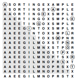 Figure 2 Selection sort example
The first pass has no effect in this example, because there is no element in the array smaller than the A at the left. On the second pass, the other A is the smallest remaining element, so it is exchanged with the S in the second position. Then, the E near the middle is exchanged with the O in the third position on the third pass; then, the other E is exchanged with the R in the fourth position on the fourth pass; and so forth.
Program 2 Selection sort
For each i from l to r – 1, exchange a[ i ] with the minimum element in a[ i ], . . . , a[r]. As the index i travels from left to right, the elements to its left are in their final position in the array (and will not be touched again), so the array is fully sorted when i reaches the right end.

Program 2 is an implementation of selection sort that adheres to our conventions. The inner loop is just a comparison to test a current element against the smallest element found so far (plus the code necessary to increment the index of the current element and to check that it does not exceed the array bounds); it could hardly be simpler. The work of moving the items around falls outside the inner loop: each exchange puts an element into its final position, so the number of exchanges is N – 1 (no exchange is needed for the final element). Thus the running time is dominated by the number of comparisons. In later section, we show this number to be proportional to N², and examine more closely how to predict the total running time and how to compare selection sort with other elementary sorts.
A disadvantage of selection sort is that its running time depends only slightly on the amount of order already in the file. The process of finding the minimum element on one pass through the file does not seem to give much information about where the minimum might be on the next pass through the file. For example, the user of the sort might be surprised to realize that it takes about as long to run selection sort for a file that is already in order, or for a file with all keys equal, as it does for a randomly ordered file! As we shall see, other methods are better able to take advantage of order in the input file.
Despite its simplicity and evident brute-force approach, selection sort outperforms more sophisticated methods in one important application: it is the method of choice for sorting files with huge items and small keys. For such applications, the cost of moving the data dominates the cost of making comparisons, and no algorithm can sort a file with substantially less data movement than selection sort.
3、Insertion Sort
The method that people often use to sort bridge hands is to consider the elements one at a time, inserting each into its proper place among those already considered (keeping them sorted). In a computer implementation, we need to make space for the element being inserted by moving larger elements one position to the right, and then inserting the element into the vacated position. The sort function in Program 1 is an implementation of this method, which is called insertion sort.
As in selection sort, the elements to the left of the current index are in sorted order during the sort, but they are not in their final position, as they may have to be moved to make room for smaller elements encountered later. The array is, however, fully sorted when the index reaches the right end. Figure 3 shows the method in operation on a sample file.
 Figure 3 Insertion sort example
During the first pass of insertion sort, the S in the second position is larger than the A, so it does not have to be moved. On the second pass, when the O in the third position is encountered, it is exchanged with the S to put A O S in sorted order, and so forth. Unshaded elements that are not circled are those that were moved one position to the right.
The implementation of insertion sort in Program 1 is straight-forward, but inefficient. We shall now consider three ways to improve it, to illustrate a recurrent theme throughout many of our implementations: We want code to be succinct, clear, and efficient, but these goals sometimes conflict, so we must often strike a balance. We do so by developing a natural implementation, then seeking to improve it by a sequence of transformations, checking the effectiveness (and correctness) of each transformation.
First, we can stop doing compexch operations when we encounter a key that is not larger than the key in the item being inserted, because the subarray to the left is sorted. Specifically, we can break out of the inner for loop in sort in Program 1 when the condition less(a[ j – 1 ], a[ j ]) is true. This modification changes the implementation into an adaptive sort, and speeds up the program by about a factor of 2 for randomly ordered keys (see Property 2 in Sorting~Elementary Sorting Methods II).
With the improvement described in the previous paragraph, we have two conditions that terminate the inner loop——we could recode it as a while loop to reflect that fact explicitly. A more subtle improvement of the implementation follows from noting that the test j > 1 is usually extraneous: indeed, it succeeds only when the element inserted is the smallest seen so far and reaches the beginning of the array. A commonly used alternative is to keep the keys to be sorted in a[1] to a[N], and to put a sentinel key in a[0], making it at least as small as the smallest key in the array. Then, the test whether a smaller key has been encountered simultaneously tests both conditions of interest, making the inner loop smaller and the program faster.
Sentinels are sometimes inconvenient to use: perhaps the smallest possible key is not easily defined, or perhaps the calling routine has no room to include an extra key. Program 3 illustrates one way around these two problems for insertion sort: We make an explicit first pass over the array that puts the item with the smallest key in the first position. Then, we sort the rest of the array, with that first and smallest item now serving as sentinel. We generally shall avoid sentinels in our code, because it is often easier to understand code with explicit tests, but we shall note situations where sentinels might be useful in making programs both simpler and more efficient.
Program 3 Insertion sort
This code is an improvement over the implementation of sort in Program 1 because ( i ) it first puts the smallest element in the array into the first position, so that that element can serve as a sentinel; ( ii ) it does a single assignment, rather than an exchange, in the inner loop; and ( iii ) it terminates the inner loop when the element being inserted is in position. For each i, it sorts the elements a[ l ], . . . , a[ i ] by moving one position to the right elements in the sorted list a[ l ], . . . , a[ i – 1 ] that are larger than a[ i ], then putting a[ i ] into its proper position.
![]()
The third improvement that we shall consider also involves removing extraneous instructions from the inner loop. It follows from noting that successive exchanges involving the same element are inefficient. If there are two or more exchanges, we have![]() followed by
followed by![]() and so forth. The value of t does not change between these two sequences, and we waste time storing it, then reloading it for the next exchange. Program 3 moves larger elements one position to the right instead of using exchanges, and thus avoids wasting time in this way. Program 3 is an implementation of insertion sort that is more efficient than the one given in Program 1. In this series, we are interested both in elegant and efficient algorithms and in elegant and efficient implementations of them. In this case, the underlying algorithms do differ slightly——we should properly refer to the sort function in Program 1 as a nonadaptive insertion sort. A good understanding of the properties of an algorithm is the best guide to developing an implementation that can be used effectively in an application.
and so forth. The value of t does not change between these two sequences, and we waste time storing it, then reloading it for the next exchange. Program 3 moves larger elements one position to the right instead of using exchanges, and thus avoids wasting time in this way. Program 3 is an implementation of insertion sort that is more efficient than the one given in Program 1. In this series, we are interested both in elegant and efficient algorithms and in elegant and efficient implementations of them. In this case, the underlying algorithms do differ slightly——we should properly refer to the sort function in Program 1 as a nonadaptive insertion sort. A good understanding of the properties of an algorithm is the best guide to developing an implementation that can be used effectively in an application.
Unlike that of selection sort, the running time of insertion sort primarily depends on the initial order of the keys in the input. For example, if the file is large and the keys are already in order (or even are nearly in order), then insertion sort is quick and selection sort is slow.
4、Bubble Sort
The first sort that many people learn, because it is so simple, is bubble sort: Keep passing through the file, exchanging adjacent elements that are out of order, continuing until the file is sorted. Bubble sort’s prime virtue is that it is easy to implement, but whether it is actually easier to implement than insertion or selection sort is arguable. Bubble sort generally will be slower than the other two methods, but we consider it briefly for the sake of completeness.
Suppose that we always move from right to left through the file. Whenever the minimum element is encountered during the first pass, we exchange it with each of the elements to its left, eventually putting it into position at the left end of the array. Then on the second pass, the second smallest element will be put into position, and so forth. Thus, N passes suffice, and bubble sort operates as a type of selection sort, although it does more work to get each element into position. Program 4 is an implementation, and Figure 4 shows an example of the algorithm in operation.
 Figure 4 Bubble sort example
Small keys percolate over to the left in bubble sort. As the sort moves from right to left, each key is exchanged with the one on its left until a smaller one is encountered. On the first pass, the E is exchanged with the L, the P, and the M before stopping at the A on the right; then the A moves to the beginning of the file, stopping at the other A, which is already in position. The ith smallest key reaches its final position after the ith pass, just as in selection sort, but other keys are moved closer to their final position, as well.
Program 4 Bubble sort
For each i from l to r-1, the inner ( j ) loop puts the minimum element among the elements in a[ i ], . . . , a[ r ] into a[ i ] by passing from right to left through the elements, compare-exchanging successive elements. The smallest one moves on all such comparisons, so it “bubbles” to the beginning. As in selection sort, as the index i travels from left to right through the file, the elements to its left are in their final position in the array.
![]()
We can speed up Program 4 by carefully implementing the inner loop, in much the same way as we did in Section 3 for insertion sort. Indeed, comparing the code, Program 4 appears to be virtually identical to the nonadaptive insertion sort in Program 1. The difference between the two is that the inner for loop moves through the left (sorted) part of the array for insertion sort and through the right (not necessarily sorted) part of the array for bubble sort.
Program 4 uses only compexch instructions and is therefore nonadaptive, but we can improve it to run more efficiently when the file is nearly in order by testing whether no exchanges at all are performed on one of the passes (and therefore the file is in sorted order, so we can break out of the outer loop). Adding this improvement will make bubble sort faster on some types of files, but it is generally not as effective as is changing insertion sort to break out of the inner loop.