
In Recursion and Trees~ Recursive Algorithms we have discussed the relationship between mathematical recurrences and simple recursive programs, and we consider a number of examples of practical recursive programs. In this article we examine the fundamental recursive scheme known as divide and conquer, which we use to solve fundamental problems in several later sections.
Many of the recursive programs that we consider in this series use two recursive calls, each operating on about one-half of the input. The recursive scheme is perhaps the most important instance of the well-known divide-and-conquer paradigm for algorithm design, which serves as the basis for many of our most important algorithms. As an example, let us consider the task of finding the maximum among N items stored in an array a[0], . . . , a[N – 1]. We can easily accomplish this task with a single pass through the array, as follows:![]() The recursive divide-and-conquer solution given in Program 1 is also a simple (entirely different) algorithm for the same problem; we use it to illustrate the divide-and-conquer concept. More often, we use the divide-and-conquer approach because it provides solutions faster than those available with simple iterative algorithms, but it also is worthy of close examination as a way of understanding the nature of certain fundamental computations.
The recursive divide-and-conquer solution given in Program 1 is also a simple (entirely different) algorithm for the same problem; we use it to illustrate the divide-and-conquer concept. More often, we use the divide-and-conquer approach because it provides solutions faster than those available with simple iterative algorithms, but it also is worthy of close examination as a way of understanding the nature of certain fundamental computations.
Program 1 Divide-and-conquer to find the maximum
The function divides a file a[1], . . . , a[r] into a[l], . . . , a[m] and a[m+1], . . . , a[r], find the maximum elements in the two parts (recursively), and return the larger of the two as the maximum element in the whole file. It assumes that Item is a first-class type for which > is defined. If the file size is even, the two parts are equal in size; if the file size if odd, the size of the first part is 1 greater than the size of the second part.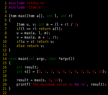
![]()
Figure 1 shows the recursive calls that are made when Program 1 is invoked for a sample array. The underlying structure seems complicated, but we normally do not need to worry about it—we depend on a proof by induction that the program works, and we use a recurrence relation to analyze the program’s performance.
 Figure 1 A recursive approach to finding the maximum
This sequence of function calls illustrates the dynamics of finding the maximum with a recursive algorithm.
As usual, the code itself suggests the proof by induction that it performs the desired computation:
- It finds the maximum for arrays of size 1 explicitly and immediately.
- For N > 1, it partitions the array into two arrays of size less than N, finds the maximum of the two parts by the inductive hypothesis, and returns the larger of these two values, which must be the maximum value in the whole array.
Moreover, we can use the recursive structure of the program to understand its performance characteristics.
Property 1 A recursive function that divides a problem of size N into two independent (nonempty) parts that it solves recursively calls itself less than N times.
If the parts are one of size k and one of size N-k, then the total number of recursive function calls that we use is ![]() The solution Tn = N – 1 is immediate by induction. If the sizes sum to a value less than N, the proof that the number of calls is less than N-1 follows the same inductive argument. Program 1 is representative of many divide-and-conquer algorithms with precisely the same recursive structure, but other examples may differ in two primary respects. First, Program 1 does a constant amount of work on each function call, so its total running time is linear. Other divide-and-conquer algorithms may perform more work on each function call, as we shall see, so determining the total running time requires more intricate analysis. The running time of such algorithms depends on the precise manner of division into parts. Second, Program 1 is representative of divide-and-conquer algorithms for which the parts sum to make the whole. Other divide-and-conquer algorithms may divide into smaller parts that total up to more than the whole problem. These algorithms are still proper recursive algorithms because each part is smaller than the whole, but analyzing them is more difficult than analyzing Program 1. We shall consider the analysis of these different types of algorithms in detail as we encounter them.
The solution Tn = N – 1 is immediate by induction. If the sizes sum to a value less than N, the proof that the number of calls is less than N-1 follows the same inductive argument. Program 1 is representative of many divide-and-conquer algorithms with precisely the same recursive structure, but other examples may differ in two primary respects. First, Program 1 does a constant amount of work on each function call, so its total running time is linear. Other divide-and-conquer algorithms may perform more work on each function call, as we shall see, so determining the total running time requires more intricate analysis. The running time of such algorithms depends on the precise manner of division into parts. Second, Program 1 is representative of divide-and-conquer algorithms for which the parts sum to make the whole. Other divide-and-conquer algorithms may divide into smaller parts that total up to more than the whole problem. These algorithms are still proper recursive algorithms because each part is smaller than the whole, but analyzing them is more difficult than analyzing Program 1. We shall consider the analysis of these different types of algorithms in detail as we encounter them.
For example, the binary-search algorithm that we studied in Principles of Algorithm Analysis II is a divide-and-conquer algorithm that divides a problem in half, then works on just one of the halves. Figure 2 indicates the contents of the internal stack maintained by the programming environment to support the computation in Figure 1. The model depicted in the figure is idealistic, but it gives useful insights into the structure of the divide-and-conquer computation. If a program has two recursive calls, the actual internal stack contains one entry corresponding to the first function call while that function is being executed (which contains values of arguments, local variables, and a return address), then a similar entry corresponding to the second function call while that function is being executed. The alternative that is depicted in Figure 2 is to put the two entries on the stack at once, keeping all the subtasks remaining to be done explicitly on the stack. This arrangement plainly delineates the computation, and sets the stage for more general computational schemes.
 Figure 2 Example of internal stack dynamics
This sequence is an idealistic representation of the contents of the internal stack during the sample computation of Figure 1. We start with the left and right indices of the whole subarray on the stack. Each line depicts the result of popping two indices and, if they are not equal, pushing four indices, which delimit the left subarray and the right subarray after the popped subarray is divided into two parts. In practice, the system keeps return address and local variables on the stack, instead of this specific representation of the work to be done, but this model suffices to describe the computation.
Figure 3 depicts the structure of the divide-and-conquer find-the-maximum computation. It is a recursive structure: the node at the top contains the size of the input array, the structure for the left subarray is drawn at the left and the structure for the right subarray is drawn at the right. We will formally define and discuss tree structures of this type in later sections. They are useful for understanding the structure of any program involving nested function calls—recursive programs in particular. Also shown in Figure 3 is the same tree, but with each node labeled with the return value for the corresponding function call. In later section, we shall consider the process of building explicit linked structure that represent trees like this one.
 Figure 3 Recursive structure of find-the-maximum algorithm.
The divide-and-conquer algorithm splits a problem of size 11 into one of size 6 and one of size 5, a problem of size 6 into two problems of size 3, and so forth, until reaching problems of size 1 (top). Each circle in these diagrams represents a call on the recursive function, to the nodes just below connected to it by lines (squares are those calls for which the recursion terminates). The diagram in the middle shows the value of the index into the middle of the file that we use to effect the split; the diagram at the bottom shows the return value.
No discussion of recursion would be complete without the ancient towers of Hanoi problem. The disks differ in size, and are initially arranged on one of the pegs, in order from largest (disk N) at the bottom to smallest (disk 1) at the top. The task is to move the stack of disks to the right one position (peg), while obeying the following rules: ( i ) only one disk may be shifted at a time; and ( ii ) no disk may be placed on top of a smaller one. One legend says that the world will end when a certain group of monks accomplishes this task in a temple with 40 golden disks on three diamond pegs.
Program 2 gives a recursive solution to the problem. It specifies which disk should be shifted at each step, and in which direction (+ means move one peg to the right, cycling to the leftmost peg when on the rightmost peg; and – means move one peg to the left, cycling to the rightmost peg when on the leftmost peg). The recursion is based on the following idea: To move N disks one peg to the right, we first move the top N-1 disks one peg to the left, then shift disk N one peg to the right, then move the N-1 disks one more peg to the left (onto disk N). We can verify that this solution works by induction. Figure 4 shows the moves for N = 5 and the recursive calls for N = 3. An underlying pattern is evident, which we now consider in detail.
 Figure 4 Towers of Hanoi
This diagram depicts the solution of the towers of Hanoi problem for five disks. We shift the top four disks left one position (left column), then move disk 5 to the right, then shift the top four disks left one position (right column). The sequence of function calls that follows constitutes the computation for three disks. The computed sequence of moves is +1, -2, +1, +3, +1, -2, +1, which appears four times in the solution (for example, the first seven moves).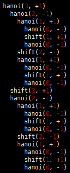 Program 2 Solution to the towers of Hanoi
We shift the tower of disks to the right by (recursively) shifting all but the bottom disk to the left, then shifting the bottom disk to the right, then (recursively) shifting the tower back onto the bottom disk.
First, the recursive structure of this solution immediately tells us the number of moves that the solution requires.
Property 2 The recursive divide-and-conquer algorithm for the towers of Hanoi problem produces a solution that has ![]() moves.
moves.
As usual, it is immediate from the code that the number of moves satisfies a recurrence. In this case, the recurrence satisfied by the number of disk moves is similar to Formula 5 in Principles of Algorithm Analysis I:![]() We can verify the stated result directly by induction: we have
We can verify the stated result directly by induction: we have![]() and, if
and, if![]() then
then![]() If the monks are moving disks at the rate of one per second, it will take at least 348 centuries for them to finish (see Figure 5), assuming that they do not make a mistake. The end of the world is likely be even further off than that because those monks presumably never have had the benefit of being able to use Program 2, and might not be able to figure out so quickly which disk to move next. We now consider an analysis of the method that leads to a simple (nonrecursive) method that makes the decision easy. While we may not wish to let monks in on the secret, it is relevant to numerous important practical algorithms.
If the monks are moving disks at the rate of one per second, it will take at least 348 centuries for them to finish (see Figure 5), assuming that they do not make a mistake. The end of the world is likely be even further off than that because those monks presumably never have had the benefit of being able to use Program 2, and might not be able to figure out so quickly which disk to move next. We now consider an analysis of the method that leads to a simple (nonrecursive) method that makes the decision easy. While we may not wish to let monks in on the secret, it is relevant to numerous important practical algorithms.
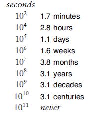 Figure 5 Seconds conversions
The vast difference between number such as 10000 and 100000000 is more obvious when we consider them to measure time in seconds and convert to familiar units of time.
To understand the towers of Hanoi solution, let us consider the simple task of drawing the markings on a ruler. Each inch on the ruler has a mark at the 1/2 inch point, slightly shorter marks at 1/4 inch intervals, still shorter marks at 1/8 inch intervals, and so forth. Our task is to write a program to draw these marks at any given resolution, assuming that we have at our disposal a procedure mark(x, h) to make a mark h units high at position x.
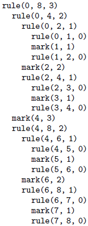
If the desired resolution is (1/2)n inches, we rescale so that our task is to put a mark at every point between 0 and (2)n, endpoints not included. Thus, the middle mark should be n units high, the marks in the middle of the left and right halves should be n – 1 units high, and so forth. Program 3 is a straightforward divide-and-conquer algorithm to accomplish this objective; Figure 6 illustrates it in operation on a small example. Recursively speaking, the idea behind the method is the following. To make the marks in an interval, we first divide the interval into two equal halves. Then, we make the (shorter) marks in the left half (recursively), the long mark in the middle, and the (shorter) marks in the right half (recursively). Iteratively speaking, Figure 6 illustrates that the method makes the marks in order, from left to right——the trick lies in computing the lengths. The recursion tree in the figure helps us to understand the computation: Reading down, we see that the length of the mark decreases by 1 for each recursive function call. Reading across, we get the marks in the order that they are drawn, because, for any given node, we first draw the marks associated with the function call on the left, then the mark associated with the node, then the marks associated with the function call on the right.
Program 3 Divide and conquer to draw a ruler
To draw the marks on a ruler, we draw the marks on the left half, then draw the longest mark in the middle, then draw the marks on the right half. This program is intended to be used with r — l equal to a power of 2—a property that it preserves in its recursive calls. Figure 6 Ruler-drawing function calls
This sequence of function calls constitutes the computation for drawing a ruler of length 8, resulting in marks of lengths 1, 2, 1, 3, 1, 2, and 1.
We see immediately that the sequence of lengths if precisely the same as the sequence of disks moved for the towers of Hanoi problem. Indeed, a simple proof that they are identical is that the recursive programs are the same. Put another way, our monks could use the marks on a ruler to decide which disk to move. Moreover, both the towers of Hanoi in Program 2 and the ruler-drawing program in Program 3 are variants of the basic divide-and-conquer scheme exemplified by Program 1. All three solve a problem of size (2)n by dividing it into two problems of size (2)n-1. For finding the maximum, we have a linear-time solution in the size of the input; for drawing a ruler and for solving the towers of Hanoi, we have a linear-time solution in the size of the output. For the towers of Hanoi, we normally think of the solution as being exponential time, because we measure the size of the problem in terms of the number of disks, n.
It is easy to draw the marks on a ruler with a recursive program, but is there some simpler way to compute the length of the i th mark, for any given i ? Figure 7 shows yet another simple simple computational process that provides the answer to this question. The i th number printed out by both the towers of Hanoi program and the ruler program is nothing other than the number of trailing 0 bits in the binary representation of i. We can prove this property by induction by correspondence with a divide-and-conquer formulation for the process of printing the table of n-bit numbers: Print the table of (n – 1)-bit numbers, each preceded by a 0 bit, then print the table of (n – 1)-bit numbers each preceded by a 1-bit.
 Figure 7 Binary counting and the ruler function
Computing the ruler function is equivalent to counting the number of trailing zeros in the even N-bit numbers.
For the towers of Hanoi problem, the implication of the correspondence with n-bit numbers is a simple algorithm for the task. We can move the pile one peg to the right by iterating the following two steps until done:
- Move the small disk to the right if n is odd (left if n is even).
- Make the only legal move not involving the small disk.
That is, after we move the small disk, the other two pegs contain two disks, one smaller than the other. The only legal move not involving the small disk is to move the smaller one onto the larger one. Every other move involves the small disk for the same reason that every other number is odd and that every other mark on the rule is the shortest. Perhaps our monks do know this secret, because it is hard to imagine how they might be deciding which moves to make otherwise.
A formal proof by induction that every other move in the towers of Hanoi solution involves the small disk (beginning and ending with such moves) is instructive: For n = 1, there is just one move, involving the small disk, so the property holds. For n > 1, the assumption that the property holds for n – 1 implies that it holds for n by the recursive construction: The first solution for n – 1 begins with a small-disk move, and the second solution for n – 1 ends with a small-disk move, so the solution for n begins and ends with a small-disk move. We put a move not involving the small disk in between two moves that do involve the small disk (the move ending the first solution for n – 1 and the move beginning the second solution for n – 1), so the property that every other move involves the small disk is preserved.
Program 4 is an alternate way to draw a ruler that is inspired by the correspondence to binary numbers (see Figure 8). We refer to this version of the algorithm as a bottom-up implementation. It is not recursive, but it is certainly suggested by the recursive algorithm. This correspondence between divide-and-conquer algorithms and the binary representations of numbers often provides insights for analysis and development of improved versions, such as bottom-up approaches. We consider this perspective to understand, and possibly to improve, each of the divide-and-conquer algorithms that we examine.
Program 4 Nonrecursive program to draw a ruler
In constrast to Program 3, we can also draw a ruler by first drawing all the marks of length 1, then drawing all the marks of length 2, and so forth. The variable t carries the length of the marks and the variable j carries the number of marks in between two successive marks of length t. The outer for loop increments t and preserves the property j = (2)t-1. The inner for loop draws all the marks of length t. Figure 8 Drawing a ruler in bottom-up order
To draw a ruler nonrecursively, we alternate drawing marks of length 1 and skipping positions, then alternate drawing marks of length 2 and skipping remaining positions, then alternate drawing marks of length 3 and skipping remaining positions, and so forth.
The bottom-up approach involves rearranging the order of the computation when we are drawing a ruler. Figure 9 shows another example, where we rearrange the order of the three function calls in the recursive implementation. It reflects the recursive computation in the way that we first described it: Draw the middle mark, then draw the left half, then draw the right half. The pattern of drawing the marks is complex, but is the result of simply exchanging two statements in Program 3. As we shall see in later section, the relationship between Figures 6 and Figure 9 is akin to the distinction between postfix and prefix in arithmetic expressions.
Drawing the marks in order as in Figure 6 might be preferable to doing the rearranged computations contained in Program 4 and indicated in Figure 9, because we can draw an arbitrarily long ruler, if we imagine a drawing device that simply moves on to the next mark in a continuous scroll. Similarly, to solve the towers of Hanoi problem, we are constrained to produce the sequence of disk moves in the order that they are to be performed. In general, many recursive programs depend on the subproblems being solved in a particular order. For other computations (see, for example, Program 1), the order in which we solve the subproblems is irrelevant. For such computations, the only constraint is that we must solve the subproblems before we can solve the main problem. Understanding when we have the flexibility to reoreder the computation not only is a secret to success in algorithm design, but also has direct practical effects in many contexts. For example, this manner is critical when we consider implementing algorithms on parallel processors.

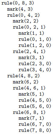 Figure 9 Ruler-drawing function calls (preorder version)
This sequence indicates the result of drawing marks before the recursive calls, instead of in between them.
The bottom-up approach corresponds to the general method of algorithm design where we solve a problem by first solving trivial subproblems, then combining those solutions to solve slightly bigger subproblems, and so forth, until the whole problem is solved. This approach might be called combine and conquer.
It is a small step from drawing rulers to drawing two-dimensional patterns such as Figure 10. This figure illustrates how a simple recursive description can lead to a computation that appears to be complex. Recursively defined geometric patterns such as Figure 10 are sometimes called fractals. If more complicated drawing primitives are used, and more complicated recursive invocations are involved (especially including recursively-defined functions on reals and in the complex plane), patterns of remarkable diversity and complexity can be developed. Another example, demonstrated in Figure 11, is the Koch star, which is defined recursively as follows: A Koch star of order 0 is the simple hill example of Figure 3 in Abstract Data Types~Stack ADT, and a Koch star of order n is a Koch star of order n – 1 with each line segment replaced by the star of order 0, scaled appropriately.
 Figure 10 Two-dimensional fractal star
This fractal is a two-dimensional version of Figure 8. The outlined boxes in the bottom diagram highlight the recursive structure of the the computation.
 Figure 11 Recursive PostScript for Koch fractal
This modification to the PostScript program of Figure 3 transforms the output into a fractal (see text).
Like the ruler-drawing and the towers of Hanoi solutions, these algorithms are linear in the number of steps, but that number is exponential in the maximum depth of the recursion. They also can be directly related to counting in an appropriate number system. The towers of Hanoi problem, ruler-drawing problem, and fractals are assuming; and the connection to binary numbers is surprising, but our primary interest in all of these topics is that they provide us with insights in understanding the basic algorithm design paradigm of divide in half and solve one or both halves independently, which is perhaps the most important such technique that we consider in this series. Table 1 includes details about binary search and mergesort, which not only are important and widely used practical algorithms, but also exemplify the divide-and-conquer algorithm design paradigm.
Table 1 Basic divide-and-conquer algorithms
Binary search and mergesort are prototypical divide-and-conquer algorithms that provide guaranteed optimal performance for searching and sorting, respectively. The recurrences indicate the nature of the divide-and-conquer computation for each algorithm. Binary search splits a problem in half, does 1 comparison, then makes a recursive call for one of the halves. Mergesort splits a problem in half, then works on both halves recursively, then does N comparisons. Throughout the series, we shall consider numerous other algorithms developed with these recursive schemes.
Quicksort and binary-tree search represent a significant variation on the basic divide-and-conquer theme where the problem is split into subproblem of size k – 1 and N – k, for some value k, which is determined by the input. For random input, these algorithms divide a problem into subproblems that are half the size (as in mergesort or in binary search) on the average. We study the analysis of the effects of this difference when we discuss these algorithms.
Other variations on the basic theme that are worthy of consideration include these: divide into parts of varying size, divide into more than two parts, divide into overlapping parts, and do various amounts of work in the nonrecursive part of the algorithm. In general, divide-and-conquer algorithms involve doing work to split the input into pieces, or to merge the results of processing two independent solved portions of input, or to help things along after half of the input has been processed. That is, there may be code before, after, or in between the two recursive calls. Naturally, such variations lead to algorithms more complicated than are binary search and mergesort, and are more difficult to analyze.